Average B predictors and the variance of the average is rho sigma squared plus (1 - rho) sigma squared over B. Derive it, see why a shared error never averages away, and compute how often a majority vote of independent classifiers is right.
ML02.2.1L2 Intermediate25 minIn review (what this means)
The maths and code on this page are checked by automated tests on every change, but an independent reader has not signed it off yet. Spot a mistake or a confusing step? Tell us.
Derive the variance of the average of B predictors with variance σ² and pairwise correlation ρ, step by step from the variance of a sum.
Explain why averaging removes the independent part of the variance but never the shared part ρσ².
Compute with the binomial distribution the chance that a majority of B independent classifiers is right, and check it by simulation.
State the two conditions an ensemble needs: members that are good on their own and members that disagree.
The question
A single deep decision tree fits its training data perfectly, yet its predictions jump about when the data change a little. Suppose you could grow a hundred such trees and average them. How much of the jumping would disappear, and what decides how much is left?
Intuition
Think of a prediction as a number that would come out differently if the training data had come out differently. Lesson ML01.8.2 called its spread over training sets the variance of the method. A deep tree has a large one.
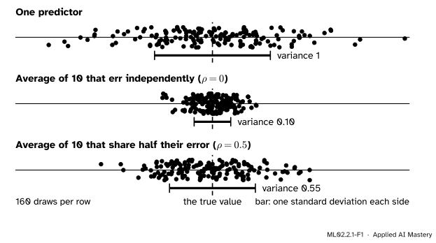
Averaging several predictions shrinks the spread, but by how much depends on whether the predictors make the same mistakes. The picture shows 160 draws of three things.
ML02.2.1-F1
Each dot is one prediction. Averaging ten predictors whose errors are independent shrinks the variance tenfold. Averaging ten whose errors are half shared barely helps: most of the spread is the shared part, and every member carries it.
When the ten errors are independent, they point in different directions and mostly cancel. When half of every error is one common error, that half is in every member, so it is in the average too. Averaging can only remove what the members do not have in common.
Build it up
Step 1. Name the parts. Take \(B\) predictors of the same target at one input. Call their predictions \(\hat{y}_1, \dots, \hat{y}_B\), each a random quantity because the training data are random. The ensemble predicts their average,
Step 2. Assume the members are alike. Each member has the same variance \(\sigma^2\), and every pair has the same correlation \(\rho\). Correlation is covariance divided by the product of the standard deviations, so every pair has covariance \(\rho\sigma^2\).
Step 3. Look at the two extremes. If \(\rho = 1\) the members are copies, the average is any one of them, and its variance stays \(\sigma^2\). If \(\rho = 0\) they are uncorrelated and the variance is \(\sigma^2/B\). The general answer has to slide between these two.
ML02.2.1-F2
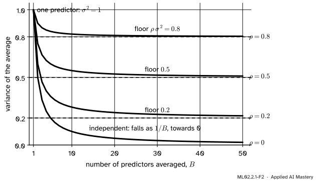
The variance of an average of \(B\) predictors, each with variance \(\sigma^2 = 1\). Every curve falls fast at first and then flattens onto its floor \(\rho\sigma^2\). Only uncorrelated members average all the way down.
Step 4. Read the curves. The first few members help most. After that each new member removes less, and nothing gets the variance below the floor. Two levers remain: lower \(\sigma^2\) (better members) or lower \(\rho\) (members that disagree). Random forests, two lessons on, pull the second lever.
The formal statement
NoteResult: variance of an average of correlated predictors
If \(\hat{y}_1, \dots, \hat{y}_B\) each have variance \(\sigma^2\) and every pair has correlation \(\rho\), then
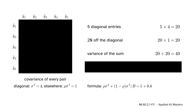
Derivation. The variance of a sum is the sum of every entry of the covariance table: the variances on the diagonal and the covariances off it (M06.10.2).
ML02.2.1-F3
The covariance table of five predictors with \(\sigma^2 = 4\) and \(\rho = 0.25\). Add up all 25 entries for the variance of the sum, then divide by \(B^2\) for the variance of the average.
The table has \(B\) cells on the diagonal, each \(\sigma^2\), and \(B^2 - B = {B(B-1)}\) cells off it, each \(\rho\sigma^2\). So
The first term does not depend on \(B\): it is the shared part, and no number of members removes it. The second shrinks like \(1/B\): it is the independent part. As \(B\) grows the variance falls to \(\rho\sigma^2\), and for \(\rho > 0\) no further.
Averaging does not change the mean of the prediction: each member has the same expected value, so the average has it too. Averaging therefore attacks variance, not bias. An ensemble of members that are all wrong in the same direction stays wrong.
Voting. Classifiers usually vote rather than average. Suppose each of \(B\) classifiers (with \(B\) odd) is right with probability \(p\) on a given input, independently of the others. The number right, \(S\), is binomial with parameters \(B\) and \(p\), and the majority is right when \(S > B/2\):
For \(p > 1/2\) the law of large numbers pushes \(S/B\) towards \(p\), which is above one half, so this chance climbs towards 1 as \(B\) grows. For \(p < 1/2\) it falls towards 0.
Go deeper: the same shared-part effect for votes
If the voters are correlated, the binomial no longer applies, and the gain shrinks just as the variance formula says. In the extreme, \(B\) copies of one classifier vote as one, and the vote is right with probability \(p\) for every \(B\). Breiman’s bound for random forests (2001, Theorem 2.3) makes the same point for votes: the error is at most \({\bar\rho\,(1 - s^2)/s^2}\), where \(s\) measures how strong each tree is and \(\bar\rho\) how correlated the trees are. Better members raise \(s\); members that disagree lower \(\bar\rho\).
Worked example
Five independent voters, each right with probability 0.6. How often is the majority right?
The majority of five is right when at least three are. Add the three binomial terms:
The total is \(0.3456 + 0.2592 + 0.07776 = 0.68256\). Five mediocre voters are right about 68 % of the time, against 60 % for one.
ML02.2.1-F4
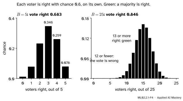
The worked example as a picture. Green bars are the outcomes where a majority is right; their heights add up to 0.683 for five voters and 0.846 for twenty-five.
With 25 voters the same sum runs from 13 to 25 and gives 0.8462. With 101 it gives 0.9791. Each voter is still only 60 % right; the crowd is 98 % right, because their mistakes are independent.
The same structure answers the variance question. With \(\sigma^2 = 4\), \(\rho = 0.25\) and \(B = 5\) (the table in the formal section), the shared part is \({0.25 \times 4} = 1\) and the independent part is \({0.75 \times 4 / 5} = 0.6\), so the average has variance 1.6 against 4 for one member. Even with infinitely many members it would stay at 1.
Code
The formula and a simulation side by side. To make predictors with correlation \(\rho\), give each one a shared normal part with weight \(\sqrt{\rho}\) and its own normal part with weight \(\sqrt{1-\rho}\).
import numpy as npfrom math import combdef variance_of_average(sigma2, rho, B):return rho * sigma2 + (1- rho) * sigma2 / Bdef correlated_predictions(sigma2, rho, B, draws, rng):"""Rows are draws; columns are B predictors with variance sigma2 and pairwise correlation rho.""" shared = rng.normal(size=(draws, 1)) own = rng.normal(size=(draws, B))return np.sqrt(sigma2) * (np.sqrt(rho) * shared + np.sqrt(1- rho) * own)rng = np.random.default_rng(0)preds = correlated_predictions(4, 0.25, 5, 200_000, rng)print("formula:", variance_of_average(4, 0.25, 5))print("simulated: member variance", preds[:, 0].var().round(2)," correlation", np.corrcoef(preds[:, 0], preds[:, 1])[0, 1].round(3)," variance of the average", preds.mean(axis=1).var().round(3))
formula: 1.6
simulated: member variance 4.01  correlation 0.248  variance of the average 1.602
Now the vote: the exact binomial sum, and a simulation of 100,000 elections for each \(B\).
def majority_right(p, B):"""Chance that more than half of B independent voters, each right with probability p, are right."""returnsum(comb(B, k) * p ** k * (1- p) ** (B - k) for k inrange(B //2+1, B +1))exact, simulated = {}, {}for B in (1, 5, 25, 101): right = rng.random((100_000, B)) <0.6# True where a voter is right exact[B] = majority_right(0.6, B) simulated[B] = (right.sum(axis=1) > B /2).mean()print(f"B = {B:3d}: exact {exact[B]:.4f}, simulated {simulated[B]:.4f}")
B =   1: exact 0.6000, simulated 0.5984
B =   5: exact 0.6826, simulated 0.6821
B =  25: exact 0.8462, simulated 0.8484
B = 101: exact 0.9791, simulated 0.9791
The simulated shares agree with the binomial to two decimals. No library call is needed here; the next lesson builds the ensemble itself.
Explore
This module’s interactive, the vote grid, lives in the next lesson. There you can add trees one at a time and watch the share of trees voting for each class settle, which is the averaging of this lesson happening cell by cell.
Pitfalls
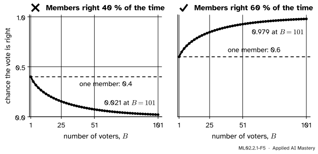
ML02.2.1-F5
Wrong beside right. A crowd of members that are worse than a coin toss votes more reliably wrong as it grows. A crowd of members that beat the coin toss votes more reliably right.
“Any crowd beats its members, so add more of them.”
Only if each member beats chance on its own. With \(p = 0.4\) the majority of 101 voters is right with probability 0.021: the vote amplifies whatever the members lean towards. An ensemble needs members that are good as well as members that disagree.
“With enough members the variance goes to zero.”
Only if the members are uncorrelated. Members trained on the same data share much of their error, so \(\rho > 0\) and the variance stops at \(\rho\sigma^2\). Fifty bagged trees with \(\rho = 0.5\) have variance \(0.5\sigma^2 + 0.01\sigma^2\), almost exactly what five hundred would have.
“Averaging also fixes a biased model.”
The average of members with the same expected value has that expected value. If every member underestimates, so does the average. Averaging is a cure for variance; lessons ML02.3 and ML02.4 build ensembles that reduce bias instead.
Check yourself
Recall
1. Write the variance of the average of \(B\) predictors with variance \(\sigma^2\) and pairwise correlation \(\rho\).
Show answer
\(\rho\sigma^2 + {(1-\rho)\sigma^2/B}\).
2. Which part of that variance does not shrink as \(B\) grows, and why?
Show answer
The shared part \(\rho\sigma^2\). It comes from the error every member has in common, so it is in the average too.
3. Five independent voters are each right with probability 0.6. What is the chance the majority is right?
Show answer
\(0.3456 + 0.2592 + 0.07776 = 0.68256\), about 0.683.
4. What happens to a majority vote of independent members that are each right with probability 0.4, as \(B\) grows?
Show answer
It becomes more and more reliably wrong: the chance it is right falls towards 0 (0.021 for \(B = 101\)).
5. Does averaging change the bias of a prediction?
Show answer
No. Members with the same expected value have an average with that expected value, so averaging reduces variance only.
Exercises
1.★ Six predictors each have variance 9 and pairwise correlation \(1/3\). Find the variance of their average, and its limit as the number of members grows.
Show solution
The shared part is \({\tfrac13 \times 9} = 3\). The independent part is \({\tfrac23 \times 9 / 6} = 6/6 = 1\). The variance of the average is \(3 + 1 = 4\). As \(B\) grows the independent part vanishes and the variance falls to 3.
2.★★ Three independent voters are each right with probability 0.7. Find the chance that the majority is right, and compare it with one voter.
Show solution
The majority of three is right when two or three are right: \({\binom{3}{2}(0.7)^2(0.3)} = 3 \times 0.49 \times 0.3 = 0.441\) and \({(0.7)^3} = 0.343\). The total is \(0.784\), against \(0.7\) for one voter.
3.★★★ Show that \(B\) quantities with a common variance \(\sigma^2 > 0\) and a common pairwise correlation \(\rho\) can exist only if \(\rho \geq {-1/(B-1)}\). What does this say about how far negative correlation can push the variance of an average down?
A variance cannot be negative, and \(B\sigma^2 > 0\), so \(1 + {(B-1)\rho} \geq 0\), which is \(\rho \geq {-1/(B-1)}\). At that limit the sum, and so the average, has variance exactly 0. For large \(B\) the limit is close to 0, so many members cannot all be strongly negatively correlated with one another; in practice ensemble members are positively correlated, and the floor \(\rho\sigma^2\) is what limits them.
Summary card
Averaging removes the errors members do not share, and only those.
ML02.2.1-F1
Independent errors cancel; shared errors stay.
Variance of an average.\(\rho\sigma^2 + {(1-\rho)\sigma^2/B}\): a floor \(\rho\sigma^2\) plus a part that shrinks like \(1/B\).
Majority vote. With independent voters right with probability \(p > 1/2\), the vote is right with a chance that climbs to 1 (0.683, 0.846, 0.979 for \(B = 5, 25, 101\) at \(p = 0.6\)).
Bias is untouched. Averaging fixes variance, not bias.
Recipe. Members that are good on their own and that disagree with each other.
Sources and next steps
Sources. Each was opened and checked against this lesson on 15 November 2026.
Trevor Hastie, Robert Tibshirani and Jerome Friedman, The Elements of Statistical Learning, 2nd edition, corrected 12th printing. Section 15.2 gives the variance of an average of identically distributed variables with pairwise correlation \(\rho\) as equation (15.1), with the derivation left as Exercise 15.1, and says that the correlation of pairs of trees limits the benefit of averaging. Section 8.7.1 gives the binomial argument for a consensus vote of independent weak learners and its caveat that bagged trees are not independent.
Leo Breiman, Random Forests, January 2001 (published in Machine Learning 45, 5 to 32). Section 2.2 and Theorem 2.3: the error of a forest is bounded by the mean correlation times \({(1 - s^2)/s^2}\), where \(s\) is the strength of the trees.
Kilian Weinberger, Lecture 18: Bagging, Cornell CS4780, Fall 2018. Bagging as a way to reduce the variance term, and why the weak law of large numbers does not apply directly to bootstrap samples, which are not independent.