The CART algorithm grows a tree by finding the best single split, then doing the same again in each child. Build it from scratch in NumPy for classes and for numbers, count what the search costs, see where greed fails, and match scikit-learn split for split.
ML02.1.3L2 Intermediate30 minIn review (what this means)
The maths and code on this page are checked by automated tests on every change, but an independent reader has not signed it off yet. Spot a mistake or a confusing step? Tell us.
State the CART recursion: best split over every feature and midpoint, recurse on both children, stop at a pure node or a limit.
Find a split in one sorted sweep and count the cost of growing a tree.
Grow a regression tree by squared-error decrease, and find the best stump of the eight-point set by hand.
Explain with the XOR pattern why a greedy tree can miss a small, perfect tree.
Write a recursive tree grower in NumPy and check it split for split against scikit-learn.
The question
The last lesson found the best first question for the twelve points. A whole tree needs more: which question to ask next on each side, and when to stop asking. Trying every possible tree is hopeless even for a few dozen points. Is there a simple rule that grows a good tree, and what does it cost to run?
From the last lesson
1. How is a candidate split scored?
Show answer
By the impurity decrease: the parent’s impurity minus the impurities of the two children, each weighted by its share of the parent’s points.
2. What is the best first split of the twelve points, and its Gini decrease?
Show answer
\(x_1 \le 3.5\), with counts 5 : 1 and 1 : 5 and a Gini decrease of \(2/9 \approx 0.222\).
Intuition
The rule is short: find the best single question, ask it, and then treat each side as a new, smaller problem of the same kind. Here it is on the twelve points, one split at a time.
ML02.1.3-F1
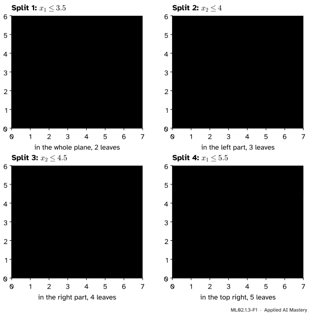
The tree of the twelve points grows split by split. Each step cuts one rectangle (yellow) with the best question for the points inside it. After four splits every rectangle is pure.
Each split is chosen by looking only at the points in one rectangle, and only one step ahead. Once made, a split is never revised. That is what greedy means: take the best move now, and do not look ahead.
Build it up
Step 1. Which thresholds to try. Between two neighbouring values of a feature, say 3 and 4, every threshold from 3 up to (but not including) 4 sends exactly the same points left. So only one threshold per gap needs testing. CART uses the midpoint, 3.5, which keeps the cut as far as possible from the training points on both sides.
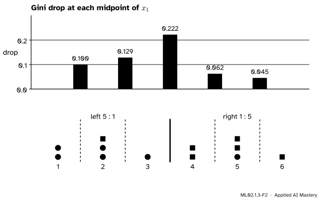
Step 2. Sweep instead of recount. Sort the points of a node by one feature and slide the threshold from left to right. Each time it passes a point, that point moves from the right child to the left child: add one to a left count and take one from a right count. Each candidate then costs one impurity evaluation, not a pass over the data.
ML02.1.3-F2
The sweep along \(x_1\) at the root. Each midpoint between neighbouring values is a candidate; the bars show its Gini drop. The same sweep runs along \(x_2\), and the best of all is kept.
Step 3. Recurse. Apply the best split, then call the same procedure on the left child and on the right child. Each call works on fewer points.
Step 4. Stop. A node becomes a leaf when it is pure, when no split is possible (all its points have the same features), or when a limit is reached. The two usual limits are a maximum depth, max_depth, and a minimum number of training points in each leaf, min_samples_leaf.
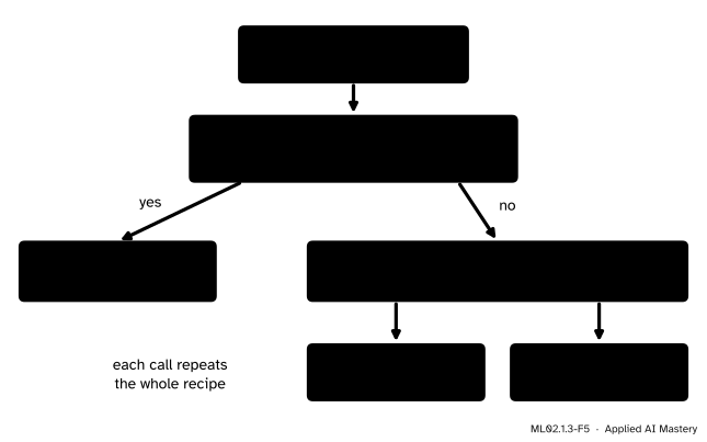
If the node is pure, or at the depth limit, or no split leaves at least min_samples_leaf points on each side, make it a leaf.
Otherwise, for each feature \(j\), sort the node’s distinct values \(u_1 < \dots < u_r\) and try each threshold \(s = {(u_i + u_{i+1})/2}\). Keep the pair \((j, s)\) with the largest impurity decrease.
Send the points with \(x_j \le s\) to the left child and the rest to the right, and call grow on each child.
ML02.1.3-F5
CART as a recursion. The only real work is the yellow box, the search for the best split.
Regression trees. For a numerical target, use the squared error of a node,
where \(\bar{y}\) is the mean target of the node (lesson 1 showed that the mean is the best leaf value). A split is scored by how much it lowers the total:
This is the impurity decrease of the last lesson with the mean squared error \({S/n}\) as the impurity, multiplied by \(n\), so both choose the same split. The sweep works here too, because \(S\) can be updated from running sums:
\[
S = \sum_i y_i^2 - \frac{1}{n}\Big(\sum_i y_i\Big)^2 .
\]
The cost. At one node with \(n\) points and \(d\) features, sorting costs about \(n \log n\) steps per feature and the sweep about \(n\). So one node costs about \(d\, n \log n\). The nodes at one depth hold disjoint sets of points, so a whole level of the tree also costs about \(d\, n \log n\), and a tree of depth \(D\) costs about \(D\, d\, n \log n\). Recounting the classes for each threshold instead would cost \(d\, n^2\) per node. Predicting is cheap: one comparison per level.
Why greedy? Finding the smallest tree that classifies the training data perfectly is NP-hard, so no fast exact method is known. The greedy rule is fast and usually good. It is also short-sighted, as the pitfalls section shows.
Worked example
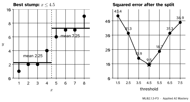
The best regression stump of the eight-point set. The targets at \(x = 1, \dots, 8\) are \(y = (1, 2, 2, 4, 6, 7, 7, 9)\), with mean \(4.75\). The squared error about the mean is \(59.5\), which is \(8 \times 7.4375\): the mean squared error of predicting \(4.75\) everywhere.
Try the threshold \(x \le 4.5\). The left leaf holds \(1, 2, 2, 4\), with mean \(2.25\); the right leaf holds \(6, 7, 7, 9\), with mean \(7.25\). The squared errors are
a total of \(9.5\), down from \(59.5\). Try \(x \le 3.5\): the left leaf \(1, 2, 2\) has mean \(5/3\) and \(S_L = 2/3\); the right leaf \(4, 6, 7, 7, 9\) has mean \(6.6\) and \(S_R = 13.2\), a total of \(13.87\). Worse. All seven thresholds:
Threshold
Left mean
Right mean
Total \(S\)
1.5
1.00
5.29
43.43
2.5
1.50
5.83
31.33
3.5
1.67
6.60
13.87
4.5
2.25
7.25
9.50
5.5
3.00
7.67
18.67
6.5
3.67
8.00
31.33
7.5
4.14
9.00
38.86
ML02.1.3-F3
The regression stump. The total squared error falls to its lowest, \(9.5\), at \(x \le 4.5\), with leaf means \(2.25\) and \(7.25\).
The best stump splits at \(4.5\). Recursing, the left leaf \(1, 2, 2, 4\) splits next at \(3.5\) and the right leaf \(6, 7, 7, 9\) at \(7.5\), which gives the staircase of lesson 1.
Code
First the classification grower. best_split sweeps each feature once; grow calls itself on the two children. A tie goes to the first split found.
import numpy as nppoints = np.array([(1, 1), (2, 1), (1, 2), (2, 3), (3, 2), (5, 5), (4, 1), (5, 2), (5, 3), (4, 4), (2, 5), (6, 5)], dtype=float)labels = np.array([0] *6+ [1] *6)def gini(counts): p = counts / counts.sum()return1- (p **2).sum()def best_split(X, y, impurity=gini, min_leaf=1): n, d = X.shape parent = impurity(np.bincount(y, minlength=2)) best = (0.0, None, None) # (decrease, feature, threshold)for j inrange(d): order = np.argsort(X[:, j], kind="stable") xs, ys = X[order, j], y[order] left = np.zeros(2) right = np.bincount(ys, minlength=2).astype(float)for i inrange(n -1): # move point i from right to left left[ys[i]] +=1 right[ys[i]] -=1if xs[i] == xs[i +1] ormin(i +1, n - i -1) < min_leaf:continue after = ((i +1) * impurity(left) + (n - i -1) * impurity(right)) / nif best[1] isNoneor parent - after > best[0] +1e-12: best = (parent - after, j, (xs[i] + xs[i +1]) /2)return bestdef grow(X, y, depth=0, max_depth=None, min_leaf=1): counts = np.bincount(y, minlength=2) node = {"counts": counts, "answer": int(np.argmax(counts))}if counts.max() ==len(y) or depth == max_depth:return node _, j, s = best_split(X, y, min_leaf=min_leaf)if j isNone:return node go = X[:, j] <= s node.update(feature=j, threshold=s, yes=grow(X[go], y[go], depth +1, max_depth, min_leaf), no=grow(X[~go], y[~go], depth +1, max_depth, min_leaf))return nodedef rules(node, depth=0):"""The splits in order, root first: (depth, feature, threshold)."""if"feature"notin node:return [] here = [(depth, node["feature"], float(node["threshold"]))]return here + rules(node["yes"], depth +1) + rules(node["no"], depth +1)tree = grow(points, labels)for depth, j, s in rules(tree):print(" "* depth +f"x{j +1} <= {s}")
x1 <= 3.5
    x2 <= 4.0
    x2 <= 4.5
        x1 <= 5.5
Now compare with scikit-learn, node for node. Its trees store thresholds in single precision, so they are compared to six decimal places. Besides the twelve points, try 200 points of the two-moons data with a depth limit of 4.
The trees agree split for split. In deeper trees two splits can tie exactly, and then the two programs may break the tie differently, so compare deep trees by their predictions, not their text.
Next, the XOR pattern of the pitfalls section. Every first split has a Gini decrease of exactly 0.
grid = np.array([(a, b) for a inrange(1, 5) for b inrange(1, 5)], dtype=float)xor = ((grid[:, 0] >2.5) ^ (grid[:, 1] >2.5)).astype(int)def predict(node, x):while"feature"in node: node = node["yes"] if x[node["feature"]] <= node["threshold"] else node["no"]return node["answer"]drop, j, s = best_split(grid, xor)print(f"first split found: x{j +1} <= {s}, Gini drop {drop:.3f}")greedy = grow(grid, xor, max_depth=2)print("greedy depth 2 right:", sum(predict(greedy, x) == t for x, t inzip(grid, xor)), "of 16")full = grow(grid, xor)print("greedy full tree:", len(rules(full)), "splits")
first split found: x1 <= 1.5, Gini drop 0.000
greedy depth 2 right: 12 of 16
greedy full tree: 5 splits
Last, the regression grower: the same sweep with running sums of \(y\) and \(y^2\).
def best_split_reg(X, y): n, d = X.shape total, total_sq = y.sum(), (y **2).sum() parent = total_sq - total **2/ n best = (0.0, None, None)for j inrange(d): order = np.argsort(X[:, j], kind="stable") xs, ys = X[order, j], y[order] s_left = sq_left =0.0for i inrange(n -1): s_left += ys[i] sq_left += ys[i] **2if xs[i] == xs[i +1]:continue k = i +1 after = (sq_left - s_left **2/ k) + ((total_sq - sq_left) - (total - s_left) **2/ (n - k))if best[1] isNoneor parent - after > best[0] +1e-12: best = (parent - after, j, (xs[i] + xs[i +1]) /2)return bestxr = np.arange(1, 9, dtype=float).reshape(-1, 1)yr = np.array([1, 2, 2, 4, 6, 7, 7, 9], dtype=float)drop, j, s = best_split_reg(xr, yr)left = yr[xr[:, 0] <= s]right = yr[xr[:, 0] > s]print(f"best stump: x <= {s}, means {left.mean()} and {right.mean()}, squared error {59.5- drop:.2f}")reg = DecisionTreeRegressor(max_depth=1).fit(xr, yr)print(export_text(reg, feature_names=["x"]))
best stump: x <= 4.5, means 2.25 and 7.25, squared error 9.50
|--- x <= 4.50
|   |--- value: [2.25]
|--- x >  4.50
|   |--- value: [7.25]
Explore
ML02.1-X1
Tree grower
Press Step to make the best next split and watch the plane and the tree diagram grow together; switch between Gini and entropy; drag a point, or pick it and move it with the sliders, and watch the tree regrow. Lower the depth slider to prune the tree back.
Things to try. Step four times and check the order against the figure above. Move the point \((2, 5)\) down to \((2, 3.5)\): the second question becomes \(x_2 \le 3.25\). Add three points of class 1 at \((1, 5)\), \((1, 4.5)\) and \((0.5, 5)\), grow fully, and watch the root question change from \(x_1 \le 3.5\) to \(x_2 \le 3.5\): a few points can change the very first question.
Pitfalls
ML02.1.3-F4
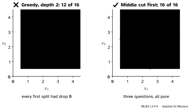
Wrong beside right on an XOR pattern. Every possible first split leaves both children half and half, so its impurity decrease is 0, and the greedy grower takes the first one it tried. The tree that starts with the middle cut is perfect after three questions.
“Greedy finds the best tree.”
It finds a good tree quickly, not the best. On XOR, no first question helps on its own, although the right first question makes a perfect tree possible. Greedy growth cannot see that, so its depth-2 tree gets 12 of 16 points right, and its full tree uses five splits where three suffice. A stopping rule of the form “stop when no split lowers the impurity” would not split XOR at all. This is one reason to grow a large tree first and prune it afterwards (lesson 4).
“The order in which I grow the nodes changes the tree.”
Not for the finished tree. Depth-first recursion and best-first growth make the same splits, because each split depends only on the points in its own node. Order matters only when you stop early by counting splits or leaves (max_leaf_nodes grows best-first).
“Thresholds can be any value between two training points.”
For the training data they can, since every such threshold makes the same split. For new data they differ: a new point between 3 and 4 is treated differently by \(x_1 \le 3.1\) and by \(x_1 \le 3.9\). The midpoint is the neutral choice, and both CART and scikit-learn use it.
Check yourself
Recall
1. Which thresholds does CART try for one feature in a node?
Show answer
The midpoints between neighbouring distinct values of that feature among the node’s points.
2. Name three reasons a node becomes a leaf.
Show answer
It is pure; it has reached max_depth; no split leaves at least min_samples_leaf points on both sides (or no split is possible at all because its points share the same features).
3. What does a regression tree use to score a split, and what does each leaf predict?
Show answer
The decrease in total squared error about the node means. Each leaf predicts the mean target of its training points.
4. About how much does it cost to find the best split in a node of \(n\) points with \(d\) features, using a sort and a sweep?
Show answer
About \(d\, n \log n\): a sort of each feature, then a linear sweep.
5. Why does a greedy grower struggle with the XOR pattern?
Show answer
Every single first split leaves both children half and half, so its impurity decrease is 0. The grower cannot see that the middle cut enables a perfect tree one level down.
Exercises
1.★ Check the row \(x \le 5.5\) of the stump table: the two means and the total squared error.
2.★★ Grow the regression tree of the eight points one more level by hand: find the best split of the left leaf \(\{1, 2, 2, 4\}\) at \(x = 1, \dots, 4\), and its leaf means.
Show solution
The three thresholds give: at \(1.5\), leaves \(\{1\}\) and \(\{2, 2, 4\}\) with errors \(0\) and \(24/9 \approx 2.67\); at \(2.5\), \(\{1, 2\}\) and \(\{2, 4\}\) with \(0.5\) and \(2\), total \(2.5\); at \(3.5\), \(\{1, 2, 2\}\) and \(\{4\}\) with \(6/9 \approx 0.67\) and \(0\). The best is \(x \le 3.5\), with leaf means \(5/3 \approx 1.67\) and \(4\), as in the staircase of lesson 1.
3.★★★ A node holds \(n\) points with \(d\) features, all values distinct. How many candidate splits does CART score at that node? If the tree is grown until every leaf holds one point, how many internal nodes does it have?
Show solution
Each feature has \(n\) distinct values and so \(n - 1\) midpoints, giving \({d(n - 1)}\) candidates. A tree whose leaves each hold one of the \(n\) points has \(n\) leaves. Each split adds one leaf to the single starting leaf, so it took \({n - 1}\) splits: the tree has \({n - 1}\) internal nodes.
Summary card
Grow a tree by taking the best split now, then repeating on each side.
ML02.1.3-F1
One rectangle cut per step.
Candidates. Each feature, each midpoint between neighbouring values.
Choice. Largest impurity decrease (classification) or squared-error decrease (regression).
Stop. Pure node, max_depth, min_samples_leaf, or no split possible.
Cost. About \(d\, n \log n\) per level; greedy, so XOR-like patterns can fool it.
Sources and next steps
Sources. Each was opened and checked against this lesson on 15 November 2026.
T. Hastie, R. Tibshirani and J. Friedman, The Elements of Statistical Learning, 2nd edition, 12th printing. Section 9.2.2: the greedy search over splitting variable and split point, equations (9.12) to (9.14), and the warning that a seemingly worthless split might lead to a very good split below it.
G. James, D. Witten, T. Hastie, R. Tibshirani and J. Taylor, An Introduction to Statistical Learning, 2nd edition. Section 8.1.1: recursive binary splitting, called top-down and greedy, with the residual sum of squares (8.3) as the criterion.
scikit-learn developers, User Guide, Section 1.10: Decision Trees (version 1.9). Section 1.10.7: the best splitter tries the midpoints between sorted distinct values; Section 1.10.4: the cost of sorting and scanning at each node; the list of disadvantages names XOR as a concept that trees do not express easily.
K. Weinberger, Cornell CS4780, lecture note 17: Decision trees. Finding a minimum-size consistent tree is NP-hard; the XOR example where the first split does not improve impurity; CART regression trees with the squared loss and the leaf average; a split search in \(O(n \log n)\).