\( \newcommand{\vect}[1]{\boldsymbol{\mathbf{#1}}} \newcommand{\mat}[1]{\boldsymbol{\mathbf{#1}}} \newcommand{\R}{\mathbb{R}} \newcommand{\E}{\mathbb{E}} \newcommand{\Prob}{\mathbb{P}} \newcommand{\T}{^{\top}} \newcommand{\norm}[1]{\lVert #1 \rVert} \newcommand{\abs}[1]{\lvert #1 \rvert} \newcommand{\ihat}{\mkern1mu\hat{\boldsymbol{\imath}}\mkern2mu} \newcommand{\jhat}{\mkern1mu\hat{\boldsymbol{\jmath}}\mkern2mu} \newcommand{\pd}[2]{\frac{\partial #1}{\partial #2}} \newcommand{\argmax}{\operatorname*{arg\,max}} \newcommand{\argmin}{\operatorname*{arg\,min}} \newcommand{\cdata}[1]{\class{c-data}{#1}} \newcommand{\cmodel}[1]{\class{c-model}{#1}} \newcommand{\ctruth}[1]{\class{c-truth}{#1}} \newcommand{\cgrad}[1]{\class{c-grad}{#1}} \newcommand{\closs}[1]{\class{c-loss}{#1}} \newcommand{\cparam}[1]{\class{c-param}{#1}} \newcommand{\csecond}[1]{\class{c-second}{#1}} \renewcommand{\,}{\mkern3mu} \)

The three libraries side by side

XGBoost, LightGBM, CatBoost and scikit-learn’s HistGradientBoosting share one objective under different names. Map their settings onto one another, see where each enters the formulas, compare them fairly on two datasets, and learn which settings to change first.

ML02.5.4L2 Intermediate30 min

In review

The maths and code on this page are checked by automated tests on every change, but an independent reader has not signed it off yet. Spot a mistake or a confusing step? Tell us.

Before this lesson: ML02.5.3 Categorical features without leakage: CatBoost's ideas

What you will be able to do

Translate the main settings of XGBoost, LightGBM, CatBoost and HistGradientBoosting into one another and into the symbols of the objective.
Derive the leaf weight under an L1 penalty as soft thresholding of G.
Compare boosting settings and a linear baseline on the same cross-validation folds, and read the fold-to-fold spread.
Choose the two or three settings to change first, and stop training early without letting the test data choose the number of rounds.

The question

A colleague sends a tuned XGBoost model with max_depth=6, min_child_weight=1 and reg_lambda=1, and asks you to rebuild it in LightGBM. LightGBM has no default depth limit, counts leaves instead, and gives min_child_weight a default a thousand times smaller. Which of its settings say the same thing, which say something else, and which matter enough to touch?

From the last lesson

1. Why does leave-one-out target encoding still leak?

Show answer

The row’s label is subtracted from its category’s total, so within a category the encoding is lower exactly when the label is 1, and a threshold can read the label off.

2. What does TargetEncoder.fit_transform do to stop a row’s label entering its encoding?

Show answer

It cross-fits: each fold of the training rows is encoded with statistics learnt on the other folds.

Intuition

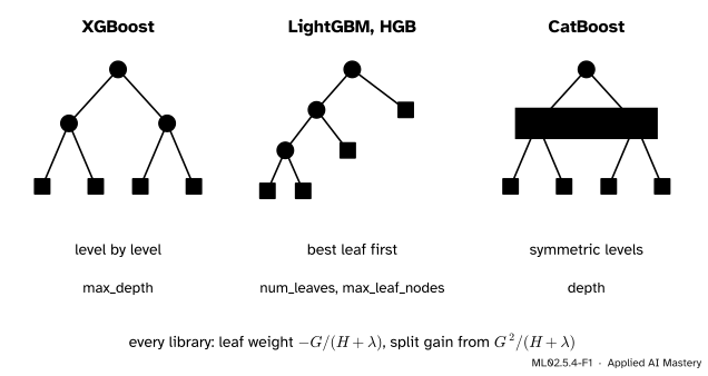
Under the brand names there is one machine: the stage objective of lesson 1, with leaf weights \({-G/(H + \lambda)}\) and split gains built from \({G^2/(H + \lambda)}\). The libraries differ in how they find splits (exactly, or on histograms), how they treat categories, and above all in the shape of the trees they grow.

ML02.5.4-F1

One objective, three tree shapes. XGBoost grows level by level to a depth; LightGBM and scikit-learn grow the best leaf first up to a number of leaves; CatBoost grows symmetric trees that ask one question per level.

So most settings are the same few dials with different names: how big a step each tree takes, how many trees, how big each tree may grow, how much each leaf is penalised, and how much data each tree sees.

Build it up

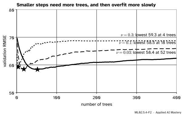
Step 1. Step size and rounds. The learning rate \(\nu\) multiplies every new tree. A smaller \(\nu\) needs more trees to reach the same fit, so the two are always set together, with the number of trees found by early stopping.

ML02.5.4-F2

The learning rate and the number of trees on one split of load_diabetes. Smaller steps reach about the same lowest error with more trees, and climb away from it more slowly, so the exact stopping point matters less.

Step 2. Tree size. Depth for XGBoost and CatBoost, number of leaves for LightGBM and scikit-learn. Deeper trees capture interactions between more features at once; they also fit noise sooner.

Step 3. What a leaf must hold. A minimum sum of Hessians in each child (min_child_weight) or a minimum number of rows. Both stop a leaf from being built on a handful of points.

Step 4. Penalties. \(\lambda\) (L2) shrinks leaf weights; \(\gamma\) is the fee per leaf; an L1 penalty \(\alpha\) moves \(G\) towards zero before dividing.

Step 5. Sampling. Each tree may see a random share of the rows (subsample) and of the columns (colsample_bytree), as in stochastic gradient boosting and random forests.

The formal statement

The settings, mapped

Names are those of each library’s scikit-learn-style interface, with documented defaults where they are fixed. A dash means the library has no such setting.

Setting	XGBoost	LightGBM	CatBoost	scikit-learn HGB
Learning rate \(\nu\)	XGBoost`learning_rate` 0.3	LightGBM`learning_rate` 0.1	CatBoost`learning_rate` (set automatically)	HGB`learning_rate` 0.1
Number of trees	XGBoost`n_estimators`	LightGBM`n_estimators` 100	CatBoost`iterations` 1000	HGB`max_iter` 100
Tree size	XGBoost`max_depth` 6	LightGBM`num_leaves` 31	CatBoost`depth` 6	HGB`max_leaf_nodes` 31
Least Hessian per leaf	XGBoost`min_child_weight` 1	LightGBM`min_child_weight` 0.001	CatBoost–	HGB–
Least rows per leaf	XGBoost–	LightGBM`min_child_samples` 20	CatBoost`min_data_in_leaf`	HGB`min_samples_leaf` 20
L2 penalty \(\lambda\)	XGBoost`reg_lambda` 1	LightGBM`reg_lambda` 0	CatBoost`l2_leaf_reg` 3	HGB`l2_regularization` 0
Fee per split \(\gamma\)	XGBoost`gamma` 0	LightGBM`min_split_gain` 0	CatBoost–	HGB–
Rows per tree	XGBoost`subsample` 1	LightGBM`subsample` 1	CatBoost`subsample`	HGB–
Columns	XGBoost`colsample_bytree` 1	LightGBM`colsample_bytree` 1	CatBoost`rsm`	HGB`max_features` 1.0
Early stopping	XGBoost`early_stopping_rounds`	LightGBM`early_stopping_round`	CatBoost`early_stopping_rounds`	HGB`early_stopping`

Notes on the table. CatBoost’s default learning rate is chosen from the data for its common losses, else \(0.03\). Its min_data_in_leaf works only with the non-symmetric growth policies. LightGBM’s subsample acts only when subsample_freq is above 0, and its max_depth is \(-1\), no limit. XGBoost can also grow best-first, with grow_policy="lossguide" and max_leaves. CatBoost’s rsm and scikit-learn’s max_features sample columns at every split, not per tree, and scikit-learn’s early stopping switches itself on above 10,000 rows. Last, a factor of 2: the code of XGBoost and LightGBM scores a split by the bracket of lesson 1 without its \(\tfrac12\), and compares gamma or min_split_gain with that number. So a fee \(\gamma\) in our formulas is gamma \(= 2\gamma\) in those libraries.

Where each setting enters. In the stage objective of lesson 1,

\[ \begin{aligned} F_m &= F_{m-1} + \cparam{\nu}\, f , \\ w_j &= -\frac{G_j}{H_j + \cparam{\lambda}} , \quad H_L, H_R \ge \cparam{m_{\text{H}}} , \\ \text{split} &\iff \text{gain}_0 > \cparam{\gamma} . \end{aligned} \]

Here \(m_{\text{H}}\) is the least Hessian per leaf, \(\text{gain}_0\) is the gain of lesson 1 before the fee \(\gamma\) is taken off, and the tree size caps the number of leaves \(T\).

The L1 penalty. Both XGBoost (reg_alpha) and LightGBM (reg_alpha) can add \(\alpha \sum_j \abs{w_j}\) to the objective. One leaf then minimises

\[ q(w) = G w + \tfrac12 (H + \lambda) w^2 + \alpha \abs{w} . \]

Write \(D = H + \lambda > 0\). Take the three cases of ML01.9.2.

If \(w > 0\): \({q'(w)} = G + D w + \alpha = 0\) gives \(w = {-(G + \alpha)/D}\), which is positive only when \(G < -\alpha\).

If \(w < 0\): \({q'(w)} = G + D w - \alpha = 0\) gives \(w = {-(G - \alpha)/D}\), which is negative only when \(G > \alpha\).

Otherwise, \(\abs{G} \le \alpha\). For \(w > 0\), \({q'(w)} = {(G + \alpha)} + Dw > 0\); for \(w < 0\), \({q'(w)} = {(G - \alpha)} + Dw < 0\). The function falls towards \(0\) from both sides, so \(w = 0\).

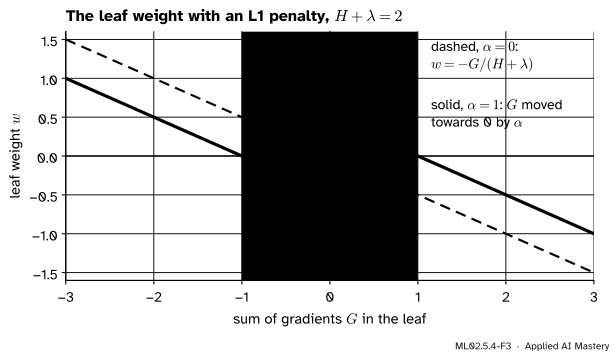
All three cases in one line, with \({S(G, \alpha)}\) the soft threshold that moves \(G\) towards zero by \(\alpha\) and stops at zero:

\[ w = -\frac{S(G, \alpha)}{H + \lambda} . \]

Putting it back, for \(G > \alpha\) with \(w = {-(G - \alpha)/D}\) (so \(\alpha\abs{w} = -\alpha w\)):

\[ \begin{aligned} q(w) &= (G - \alpha) w + \tfrac12 D w^2 \\ &= -\frac{(G - \alpha)^2}{D} + \frac12 \frac{(G - \alpha)^2}{D} \\ &= -\frac12 \frac{S(G, \alpha)^2}{H + \lambda} , \end{aligned} \]

and the case \(G < -\alpha\) is its mirror image. So the score and the gain keep their form with \(G\) replaced by \({S(G, \alpha)}\).

ML02.5.4-F3

The leaf weight under an L1 penalty, for \(H + \lambda = 2\). Without it (dashed) every leaf moves; with \(\alpha = 1\) (solid) a leaf whose \(\abs{G}\) is below \(1\) does not move at all.

Worked example

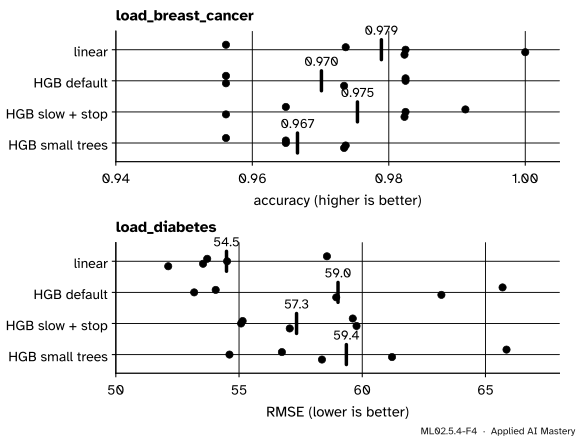
The same five folds for every model: StratifiedKFold on load_breast_cancer (569 rows, 30 features, two classes) and KFold on load_diabetes (442 rows, 10 features), both shuffled with seed 0. Four models on each: a linear model with standardised features (logistic regression or ridge with \(\lambda = 1\)), HistGradientBoosting with its defaults, the same with slow + stop (\(\nu = 0.05\), up to 1,000 trees, stopped when 20 rounds bring no gain on 15 percent of the training rows), and small trees (8 leaves, at least 10 rows each, \(\lambda = 1\)).

ML02.5.4-F4

The trace of the comparison. Dots are folds, bars are means. On both tables the spread from fold to fold is wider than the gaps between the means.

Breast cancer, accuracy. Linear \(0.979\), default \(0.970\), slow + stop \(0.975\), small trees \(0.967\). One test fold has 113 or 114 rows, so one row is worth almost \(0.009\): the four models differ by about one row per fold.

Diabetes, RMSE. Linear \(54.5\), default \(59.0\), slow + stop \(57.3\), small trees \(59.4\). Slow + stop beats the default on three folds of five and loses on two.

Reading it. Slowing down with early stopping is the one change that helped on both tables. And on these two small, clean tables a linear model is as good as any booster or better: boosting earns its place on larger tables with interactions, mixed types and missing values.

Code

import os
os.environ.setdefault("OMP_NUM_THREADS", "1")     # one thread is faster on data this small
import numpy as np
from sklearn.datasets import load_breast_cancer, load_diabetes
from sklearn.ensemble import HistGradientBoostingClassifier, HistGradientBoostingRegressor
from sklearn.linear_model import LogisticRegression, Ridge
from sklearn.model_selection import KFold, StratifiedKFold, cross_val_score
from sklearn.pipeline import make_pipeline
from sklearn.preprocessing import StandardScaler

X_bc, y_bc = load_breast_cancer(return_X_y=True)
X_db, y_db = load_diabetes(return_X_y=True)
folds_bc = StratifiedKFold(5, shuffle=True, random_state=0)
folds_db = KFold(5, shuffle=True, random_state=0)

settings = {
    "default": {},
    "slow + stop": dict(learning_rate=0.05, max_iter=1000, early_stopping=True,
                        validation_fraction=0.15, n_iter_no_change=20),
    "small trees": dict(max_leaf_nodes=8, min_samples_leaf=10, l2_regularization=1.0),
}
acc = {"linear": cross_val_score(make_pipeline(StandardScaler(), LogisticRegression()), X_bc, y_bc, cv=folds_bc)}
rmse = {"linear": -cross_val_score(make_pipeline(StandardScaler(), Ridge(1.0)), X_db, y_db, cv=folds_db,
                                   scoring="neg_root_mean_squared_error")}
for name, kw in settings.items():
    acc[name] = cross_val_score(HistGradientBoostingClassifier(random_state=0, **kw), X_bc, y_bc, cv=folds_bc)
    rmse[name] = -cross_val_score(HistGradientBoostingRegressor(random_state=0, **kw), X_db, y_db,
                                  cv=folds_db, scoring="neg_root_mean_squared_error")
for name in acc:
    print(f"{name:12s} accuracy {acc[name].mean():.3f}   RMSE {rmse[name].mean():.1f}   "
          f"RMSE by fold {np.round(rmse[name], 1)}")

linear       accuracy 0.979   RMSE 54.5   RMSE by fold [58.6 53.7 54.5 53.5 52.1]
default      accuracy 0.970   RMSE 59.0   RMSE by fold [65.7 54.1 53.2 63.2 58.9]
slow + stop  accuracy 0.975   RMSE 57.3   RMSE by fold [59.6 55.1 55.1 59.8 57.1]
small trees  accuracy 0.967   RMSE 59.4   RMSE by fold [65.9 56.7 54.6 61.2 58.4]

The scores can move in the last digit between platforms; the ranking above is what to look at. The same “slow + stop” model in the three libraries reads as follows. They are not installed in this course’s environment, so these listings are shown, not run; X_fit, y_fit and X_valid, y_valid are a training set and a validation set split off it.

import xgboost as xgb
model = xgb.XGBClassifier(learning_rate=0.05, n_estimators=1000, max_depth=6,
                          reg_lambda=1.0, early_stopping_rounds=20)
model.fit(X_fit, y_fit, eval_set=[(X_valid, y_valid)])

import lightgbm as lgb
model = lgb.LGBMClassifier(learning_rate=0.05, n_estimators=1000, num_leaves=31,
                           min_child_samples=20, early_stopping_round=20)
model.fit(X_fit, y_fit, eval_set=[(X_valid, y_valid)])

from catboost import CatBoostClassifier
model = CatBoostClassifier(learning_rate=0.05, iterations=1000, depth=6,
                           l2_leaf_reg=3, early_stopping_rounds=20, verbose=0)
model.fit(X_fit, y_fit, eval_set=(X_valid, y_valid))

Last, the soft-threshold leaf weight from the formal section, checked against a brute-force minimisation over a fine grid.

def l1_leaf_weight(G, H, lam, alpha):
    return -np.sign(G) * max(abs(G) - alpha, 0.0) / (H + lam)

grid = np.linspace(-5, 5, 200_001)
for G, H, lam, alpha in [(-3, 1, 1, 1), (-3, 1, 1, 4), (2.5, 2, 0, 0.5)]:
    q = G * grid + 0.5 * (H + lam) * grid**2 + alpha * np.abs(grid)
    print(f"G = {G}, alpha = {alpha}: formula {l1_leaf_weight(G, H, lam, alpha):.4f}, "
          f"grid {grid[np.argmin(q)]:.4f}")

G = -3, alpha = 1: formula 1.0000, grid 1.0000
G = -3, alpha = 4: formula 0.0000, grid 0.0000
G = 2.5, alpha = 0.5: formula -1.0000, grid -1.0000

What to change first. First, lower the learning rate and let early stopping on a validation split choose the number of trees. Second, the tree size, with the least number of rows per leaf. Third, \(\lambda\) and row or column sampling. Systematic search over such settings, with nested cross-validation, is the subject of ML04.5; explaining a fitted booster with SHAP values is ML04.9.

Explore

This module’s interactive is the split-gain calculator in lesson ML02.5.2. Its \(\lambda\) slider is reg_lambda of XGBoost and LightGBM and l2_regularization of scikit-learn. Its \(\gamma\) slider is half of XGBoost’s gamma or LightGBM’s min_split_gain, for the reason given under the table.

Pitfalls

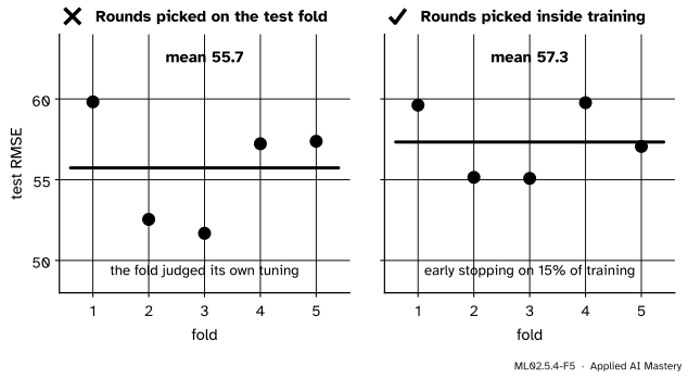
ML02.5.4-F5

Wrong beside right, on load_diabetes. Left: each fold picks the number of trees at which its own test error is lowest, and reports that error: \(55.7\), too good. Right: the number is chosen on a split of the training rows: \(57.3\), an honest estimate.

“I passed the test fold as eval_set, so early stopping used a separate set.”

The rows that chose the number of trees then also grade the model, and the score is flattered, as in the figure. Split the validation set off the training rows, inside each fold.

“Same name, same meaning.”

min_child_weight is 1 in XGBoost and 0.001 in LightGBM; \(\lambda\) is 1 in XGBoost, 0 in LightGBM and scikit-learn, and 3 in CatBoost; the learning rates start at 0.3, 0.1 and a value CatBoost picks. Copying settings across libraries without their defaults changes the model.

“num_leaves=31 is like max_depth=5.”

A full tree of depth 5 has 32 leaves. A best-first tree with 31 leaves can be up to 30 levels deep along one path. Limit both when the data are small.

“Boosting always beats a linear model on tables.”

Not on these two: the linear models scored \(0.979\) and \(54.5\). Always keep a simple baseline in the comparison.

Check yourself

Recall

1. Which setting of each library caps the size of a tree, and is it a depth or a number of leaves?

Show answer

XGBoost max_depth and CatBoost depth are depths; LightGBM num_leaves and scikit-learn max_leaf_nodes count leaves.

2. Where does \(\lambda\) appear in the leaf weight, and what are its defaults?

Show answer

In the denominator, \(w = {-G/(H + \lambda)}\). XGBoost 1, LightGBM 0, CatBoost 3 (l2_leaf_reg), scikit-learn 0.

3. What is the leaf weight under an L1 penalty \(\alpha\)?

Show answer

\(w = {-S(G, \alpha)/(H + \lambda)}\), where \(S\) moves \(G\) towards zero by \(\alpha\) and stops at zero.

4. Why are the learning rate and the number of trees set together?

Show answer

A smaller step needs more trees to reach the same fit, so the number of trees that is best depends on the learning rate. Early stopping finds it.

5. Why compare models on the same folds?

Show answer

The spread from fold to fold is often larger than the gap between models. On the same folds the differences can be read fold by fold, without the luck of the split.

Exercises

1. ★ Rewrite XGBRegressor(learning_rate=0.05, max_depth=4, reg_lambda=1.0) for HistGradientBoostingRegressor as closely as you can.

Show solution

HistGradientBoostingRegressor(learning_rate=0.05, max_depth=4, max_leaf_nodes=None, l2_regularization=1.0, min_samples_leaf=1). max_leaf_nodes=None lifts the default cap of 31 leaves so that depth alone limits the tree, as in XGBoost (a depth-4 tree has at most 16 leaves, so here the cap would not bite anyway). min_samples_leaf=1 removes the minimum of 20 rows, which XGBoost does not have; XGBoost’s min_child_weight=1 is one row under the squared loss. The trees are still grown best-first rather than level by level, but with the same depth limit.

2. ★★ A leaf has \(G = -3\), \(H = 1\) and \(\lambda = 1\). Find its weight and score for \(\alpha = 0\), \(1\) and \(4\).

Show solution

\(\alpha = 0\): \(w = 3/2 = 1.5\), score \({-\tfrac12 \cdot 9/2} = -2.25\). \(\alpha = 1\): \(S = -2\), \(w = 2/2 = 1\), score \({-\tfrac12 \cdot 4/2} = -1\). \(\alpha = 4\): \(\abs{G} = 3 \le 4\), so \(S = 0\), \(w = 0\) and score \(0\): the leaf does not move.

3. ★★★ With an L1 penalty the gain uses \({S(G, \alpha)^2}\) in place of \(G^2\). A leaf with \(G = 0\) splits into \(G_L = 0.5\) and \(G_R = -0.5\), with \(H_L = H_R = 1\) and \(\lambda = 0\). Find the gain for \(\alpha = 0\) and for \(\alpha = 1\), and explain the difference.

Show solution

\(\alpha = 0\): \({\tfrac12(0.25/1 + 0.25/1 - 0/2)} = 0.25\). \(\alpha = 1\): \({S(0.5, 1)} = {S(-0.5, 1)} = 0\) and \({S(0, 1)} = 0\), so the gain is \(0\). Both children would get weight \(0\), so the split changes no prediction and cannot lower the objective. The L1 penalty ignores gradient sums smaller than \(\alpha\), which removes splits that only chase small, noisy differences.

Summary card

Four libraries, one objective: learn the dials once.

The anchor figure again: a level-by-level tree for XGBoost, a lopsided best-leaf-first tree for LightGBM and HGB, and a symmetric tree for CatBoost, all scored with G and H. — ML02.5.4-F1
Same scores, three tree shapes.

Step and rounds. learning_rate with early stopping on a validation split.
Tree size. Depth (XGBoost, CatBoost) or leaves (LightGBM, scikit-learn), with a minimum per leaf.
Penalties. \(w = {-S(G, \alpha)/(H + \lambda)}\); split only if the gain before the fee exceeds \(\gamma\).
Compare fairly. Same folds, a linear baseline, and the fold-to-fold spread.

Sources and next steps

Sources. Each was opened and checked against this lesson on 15 November 2026.

XGBoost developers, XGBoost Parameters and the Python API reference. eta 0.3, gamma 0, max_depth 6, min_child_weight 1, subsample 1, colsample_bytree 1, lambda 1, alpha 0, grow_policy depthwise or lossguide, max_leaves; n_estimators, reg_lambda, reg_alpha and early_stopping_rounds in the scikit-learn interface.
LightGBM developers, Parameters. learning_rate 0.1, num_leaves 31, max_depth \(-1\), min_data_in_leaf 20 (alias min_child_samples), min_sum_hessian_in_leaf 0.001 (alias min_child_weight), lambda_l1 and lambda_l2 0, bagging_fraction with bagging_freq, feature_fraction, num_iterations 100, early_stopping_round, min_gain_to_split 0.
CatBoost developers, Common parameters. iterations 1000, learning_rate set automatically or 0.03, depth 6, l2_leaf_reg 3, min_data_in_leaf only for the Depthwise and Lossguide policies, rsm, subsample, and grow_policy SymmetricTree.
XGBoost and LightGBM source code, split_gain.h and feature_histogram.hpp. Both compute a leaf’s gain as \({G^2/(H + \lambda)}\), twice the fall in the objective, and LightGBM adds min_gain_to_split to the parent’s gain on that scale.
scikit-learn developers, HistGradientBoostingRegressor, scikit-learn 1.9 API reference. learning_rate 0.1, max_iter 100, max_leaf_nodes 31, min_samples_leaf 20, l2_regularization 0, max_features per split, max_bins 255, and early stopping that is on by default above 10,000 rows.

Next. This module ends here. ML02.11, Choosing a model for tabular data, compares these boosters with the other families of the course on repeated folds; ML04.5 tunes their settings systematically, and ML04.9 explains their predictions.

This lesson unlocks

ML02.11 Choosing a model for tabular data ML04.5 Hyperparameter optimization (planned) ML04.9 Interpreting models: importance, partial dependence, SHAP (planned)

Your progress is saved in this browser only. No account, no tracking.