Gaussian naive Bayes and when the assumption hurts
For measurements, give every feature of every class its own bell curve. Fit Gaussian naive Bayes to the twelve points and to iris, see why its boundary curves, then watch correlated features count the same evidence twice and push its probabilities to 0 and 1.
ML02.6.4L2 Intermediate25 minIn review (what this means)
The maths and code on this page are checked by automated tests on every change, but an independent reader has not signed it off yet. Spot a mistake or a confusing step? Tell us.
Fit Gaussian naive Bayes by maximum likelihood, one mean and one variance per feature per class, by hand and in NumPy.
Show that its decision boundary is quadratic in the features, and linear when each feature has the same variance in both classes.
Explain why correlated or duplicated features make naive Bayes overconfident while changing few of its decisions.
Describe the two regimes of Ng and Jordan: naive Bayes ahead with few examples, logistic regression ahead with many.
The question
Word counts were easy: naive Bayes just counted. What does it do with measurements, such as the petal length of a flower or the size of a tumour cell? And since its assumption is almost never true, when does that actually cost us, and how would we notice?
From the last lesson
1. In two-class multinomial naive Bayes, what is the weight of word \(j\)?
Show answer
\({w_j = \ln(\theta_{1j}/\theta_{0j})}\), the log ratio of the word’s probabilities in the two classes.
2. Why does add-one smoothing add \(V\) to the denominator?
Show answer
Every one of the \(V\) words gets one extra appearance, so the class total grows by \(V\), and the probabilities still sum to 1.
Intuition
Keep the naive assumption and change only the model of each feature. For a measurement, the simplest model is a bell curve. So each class gets one bell per feature, with its own mean and its own spread, fitted to that class’s values of that feature alone.
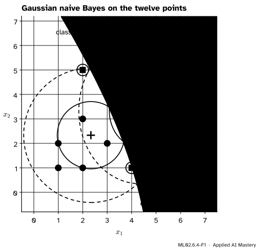
ML02.6.4-F1
Gaussian naive Bayes on the twelve points. Each class is a cloud whose contours are ellipses lined up with the axes, because the features are modelled separately. The boundary is where the two weighted clouds are equally high.
The ellipses never tilt. A tilt would mean that \(x_1\) and \(x_2\) rise and fall together within a class, and the naive model has no number for that. Lining the ellipses up with the axes is the naive assumption, drawn.
Build it up
Step 1. One bell per feature per class. Model feature \(j\) in class \(k\) as \({N(\mu_{kj}, \sigma^2_{kj})}\), a normal density with mean \(\mu_{kj}\) and variance \(\sigma^2_{kj}\).
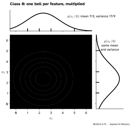
Step 2. Fit each bell by maximum likelihood. For a normal sample, the maximum-likelihood estimates are the sample mean and the average squared deviation, dividing by \(n_k\), not \({n_k - 1}\) (S02.3.3). Class 0 of the twelve points has \({x_1}\) values 1, 2, 1, 2, 3, 5. Their mean is \({14/6 = 7/3}\). Their squares sum to 44, so the variance is \({44/6 - (7/3)^2 = 17/9}\).
Step 3. Multiply the bells. Under the naive assumption the class density over the plane is the product of its feature bells.
ML02.6.4-F2
Class 0 as the product of two one-feature bells. Here both features happen to have mean 7/3 and variance 17/9, so the contours are circles.
Step 4. Score in logs and compare. As before, the score of class \(k\) is \({\ln \pi_k}\) plus the log of each feature’s bell at the new point. The class with the higher score wins.
The formal statement
NoteDefinition: Gaussian naive Bayes
For continuous features, Gaussian naive Bayes models \({p(\vect{x} \mid k) = \prod_j N(x_j;\, \mu_{kj}, \sigma^2_{kj})}\), fits \(\pi_k\) as the class share and each \(\mu_{kj}\), \(\sigma^2_{kj}\) as the mean and variance of feature \(j\) over the training examples of class \(k\), and predicts the class with the largest score
This is the special case of the class-wise Gaussian models of ML02.9 whose covariance matrices are diagonal.
The boundary is quadratic. Subtract the two scores. Expanding each square \({(x_j - \mu_{kj})^2 = x_j^2 - 2\mu_{kj}x_j + \mu_{kj}^2}\) and collecting powers of \(x_j\) gives
where \(c\) collects everything without an \(x\). The boundary \({s_1 = s_0}\) is a curve of degree two, a conic. If each feature has the same variance in both classes, every \(a_j\) is 0 and the boundary is a straight line, as in the one-feature example of ML02.6.1. On the twelve points the variances differ only a little, so the boundary bends only gently.
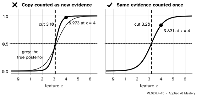
When the assumption hurts: evidence counted twice. Suppose feature 2 is an exact copy of feature 1. It carries no new information, so the true posterior is the one-feature posterior of ML02.6.1. Naive Bayes multiplies in the copy’s bell as if it were fresh evidence, so the log-likelihood ratio of the feature enters twice:
where \({\ell(x) = \ln \tfrac{p(x \mid 1)}{p(x \mid 0)}}\). With the bells \({N(2, 1)}\) and \({N(4, 1)}\), \({\ell(x) = 2x - 6}\). At \({x = 4}\) the true posterior is \({\sigma(1.595) = 0.831}\), and naive Bayes says \({\sigma(3.595) = 0.973}\). The evidence part of every log-odds is doubled, so confident answers become very confident. Decisions change only where the two log-odds have different signs: the cut moves from \({3 + \tfrac12 \ln 1.5 = 3.203}\) to \({3 + \tfrac14 \ln 1.5 = 3.101}\), because the prior now has to outweigh twice the evidence. Correlated features do the same thing in a milder form.
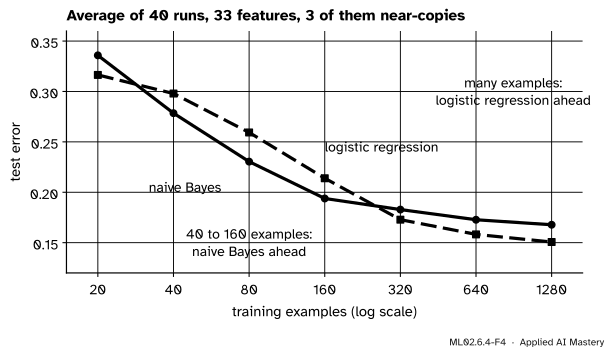
When the assumption hurts: the two regimes. Ng and Jordan compared naive Bayes with logistic regression, its discriminative twin, on 15 datasets. Naive Bayes estimates each feature’s bells on their own, from simple averages, and they showed that it settles near its best error after a number of examples that grows only with the logarithm of the number of features. That best is higher when its assumption is wrong. Logistic regression fits all its weights together and may need a number of examples that grows in proportion to the number of features, but it ends lower.
ML02.6.4-F4
The two regimes, reproduced on synthetic data where three features are near-copies of a fourth. Naive Bayes is ahead from 40 to 160 examples; logistic regression is ahead from 320 on. At 20 examples, fewer than the 33 features, logistic regression is narrowly ahead too: the regimes are a tendency, not a law.
Worked example
Fit Gaussian naive Bayes to the twelve points and classify the point \({(3, 3)}\).
Fit. Each class has six points, so \({\pi_0 = \pi_1 = 0.5}\). Class 0 has means \({(7/3,\, 7/3)}\) and variances \({(17/9,\, 17/9)}\) (Step 2). Class 1 has \(x_1\) values 4, 5, 5, 4, 2, 6, with mean \({26/6 = 13/3}\) and variance \({122/6 - (13/3)^2 = 14/9}\), and \(x_2\) values 1, 2, 3, 4, 5, 5, with mean \({20/6 = 10/3}\) and variance \({80/6 - (10/3)^2 = 20/9}\).
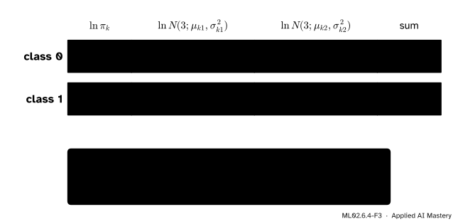
One term. The log bell of class 0’s first feature at \({x_1 = 3}\):
The other terms come the same way: \({-1.355}\) for class 0’s \(x_2\), and \({-1.711}\) and \({-1.343}\) for class 1. The point is far from class 1’s mean in \(x_1\), which costs \({(4/3)^2/(28/9) = 0.571}\).
ML02.6.4-F3
The worked example as a table of log terms. Each row adds the log prior and one log bell per feature.
Decide. The scores are \({-0.693 - 1.355 - 1.355 = -3.402}\) for class 0 and \({-0.693 - 1.711 - 1.343 = -3.748}\) for class 1. The log-odds of class 1 are \({-0.345}\), so
and the point goes to class 0. On the training points themselves the model gets 9 of 12 right; the three ringed in the anchor figure fall on the wrong side.
Code
From scratch on the twelve points, checked against GaussianNB. Its var_smoothing adds a tiny amount to every variance, \({10^{-9}}\) times the largest one, so the two agree to many decimals.
import numpy as npfrom sklearn.naive_bayes import GaussianNBX = np.array([(1, 1), (2, 1), (1, 2), (2, 3), (3, 2), (5, 5), (4, 1), (5, 2), (5, 3), (4, 4), (2, 5), (6, 5)], dtype=float)y = np.array([0] *6+ [1] *6)def fit(X, y): classes = np.unique(y) prior = np.array([np.mean(y == k) for k in classes]) mean = np.array([X[y == k].mean(axis=0) for k in classes]) var = np.array([X[y == k].var(axis=0) for k in classes]) # divides by n_kreturn prior, mean, vardef scores(X, prior, mean, var):return np.stack([np.log(prior[k]) -0.5* np.log(2* np.pi * var[k]).sum()- ((X - mean[k]) **2/ (2* var[k])).sum(axis=1) for k inrange(len(prior))], axis=1)def proba(s): e = np.exp(s - s.max(axis=1, keepdims=True))return e / e.sum(axis=1, keepdims=True)prior, mean, var = fit(X, y)print("means:", mean.round(4).tolist(), " variances:", var.round(4).tolist())p33 = proba(scores(np.array([[3.0, 3.0]]), prior, mean, var))[0, 1]train_right = (scores(X, prior, mean, var).argmax(axis=1) == y).sum()print(f"P(class 1 | (3, 3)) = {p33:.4f}; training points right: {train_right} of 12")print("GaussianNB:", GaussianNB().fit(X, y).predict_proba([[3.0, 3.0]])[0, 1].round(4))
test accuracy, ours: 0.978, GaussianNB: 0.978
largest difference in probabilities: 2.7e-08
Now the cost of the assumption, on load_breast_cancer, whose 30 features include many that move together (radius, perimeter and area, for a start). Feed naive Bayes the features once, twice and three times over, and compare with logistic regression.
naive Bayes, 1 copy: accuracy 0.924, beyond 0.01 or 0.99: 95%, log loss 1.09
naive Bayes, 2 copies: accuracy 0.924, beyond 0.01 or 0.99: 98%, log loss 1.54
naive Bayes, 3 copies: accuracy 0.924, beyond 0.01 or 0.99: 98%, log loss 1.78
logistic regression: accuracy 0.959, log loss 0.085
Accuracy does not move: 92.4% with one, two or three copies, and not one decision changes. But over nine answers in ten are already beyond 0.01 or 0.99, and the log loss, which punishes confident mistakes, grows with every copy. Logistic regression is both more accurate and far less overconfident.
Finally the two regimes of the figure above, as code: 33 features, three of them noisy copies of the first, 40 repetitions per training size, logistic regression with almost no penalty (C=1e4), as in Ng and Jordan.
import warningsdef make(n, rng): y = rng.integers(0, 2, n) z = rng.normal(size=(n, 30)) +0.4* y[:, None] # independent given the classreturn np.hstack([z, z[:, :1] +0.3* rng.normal(size=(n, 3))]), y # plus 3 near-copiesrng = np.random.default_rng(0)X_test, y_test = make(4000, rng)sizes = [20, 40, 80, 160, 320, 640, 1280]err = np.zeros((2, len(sizes)))with warnings.catch_warnings(): warnings.simplefilter("ignore")for _ inrange(40):for j, m inenumerate(sizes): Xm, ym = make(m, rng)whilemin(np.bincount(ym, minlength=2)) <2: Xm, ym = make(m, rng) err[0, j] +=1- GaussianNB().fit(Xm, ym).score(X_test, y_test) err[1, j] +=1- LogisticRegression(C=1e4, max_iter=5000).fit(Xm, ym).score(X_test, y_test)err /=40for m, nb, lr_err inzip(sizes, *err):print(f"{m:5d} examples: naive Bayes {nb:.3f}, logistic regression {lr_err:.3f}")
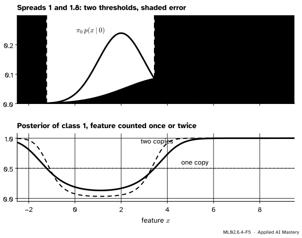
Drag the two bells, or use the sliders, to set each class’s mean and spread, and slide the prior of class 1. Watch the thresholds and the shaded error move. Then press Duplicate the feature and compare the posterior that naive Bayes reports with the true one.
Three things to try. Make the spreads equal, then unequal, and count the thresholds: one or two. Push the prior of class 1 down to 0.1 and watch the cut retreat towards class 1, as in the pitfall of ML02.6.1. With the duplicate switched on, find a value of \(x\) where the two posteriors differ by more than 0.1 but give the same decision.
Pitfalls
ML02.6.4-F6
Wrong beside right. A duplicated feature barely moves the cut, from 3.20 to 3.10, but turns 0.831 into 0.973.
“Adding another feature can only give naive Bayes more to go on.”
Not if it repeats what another feature already says. Naive Bayes multiplies in its likelihood as fresh evidence, so redundant features count the same evidence again. On the breast-cancer data, three copies of every feature leave the accuracy at 92.4% and push the log loss from 1.09 to about 1.8.
“A naive Bayes probability of 0.999 means near certainty.”
On load_breast_cancer, 95% of its answers are beyond 0.01 or 0.99, and most of its 13 mistakes are among them. The scikit-learn guide puts it plainly: naive Bayes is a decent classifier but a bad estimator, so predict_proba should not be taken too seriously. Use its ranking and decisions; when you need probabilities, calibrate them (ML04.7).
“A feature that never varies within a class is harmless.”
Its fitted variance is 0, and the bell becomes a spike: the score divides by zero. GaussianNB guards against this with var_smoothing, which adds \({10^{-9}}\) times the largest feature variance to every variance. A from-scratch version needs the same guard.
Check yourself
Recall
1. What does Gaussian naive Bayes estimate for each class?
Show answer
The prior \(\pi_k\), and for every feature a mean \(\mu_{kj}\) and a variance \(\sigma^2_{kj}\), the maximum-likelihood estimates from that class’s training examples.
2. Why do the contour ellipses of a Gaussian naive Bayes class never tilt?
Show answer
Each feature has its own bell and they are multiplied, so there is no term that links \(x_1\) and \(x_2\). A tilt would need a covariance between them.
3. When is the boundary of two-class Gaussian naive Bayes a straight line?
Show answer
When every feature has the same variance in both classes, so that each \({a_j = 0}\) and the \(x_j^2\) terms cancel.
4. A feature is duplicated. What happens to the naive log-odds, and to the decisions?
Show answer
The feature’s log-likelihood ratio is added twice, so the log-odds grow and posteriors move towards 0 and 1. Decisions change only for inputs near the threshold, where the prior and the doubled evidence now balance differently.
5. What are Ng and Jordan’s two regimes?
Show answer
With few training examples naive Bayes is usually ahead, because it approaches its best error faster. With many, logistic regression is ahead, because its best error is lower.
Exercises
1.★ Compute the log bell of class 1’s second feature at \({x_2 = 3}\) for the twelve points, and check it against the table.
Show solution
The mean is \({10/3}\) and the variance \({20/9}\). So the term is
The first part is \({-\tfrac12 \ln 13.963 = -1.318}\); the second is \({(1/9)/(40/9) = 0.025}\). The term is \({-1.318 - 0.025 = -1.343}\), as in the table.
2.★★ With the bells \({N(2, 1)}\) and \({N(4, 1)}\) and priors 0.6 and 0.4, a feature is copied \(m\) times, so naive Bayes sees it \({m + 1}\) times. Find the naive threshold, and the naive posterior at \({x = 4}\) for \({m = 2}\).
Show solution
The naive log-odds are \({\ln(2/3) + (m + 1)(2x - 6)}\). Setting them to 0 gives \({2x - 6 = \ln 1.5/(m + 1)}\), so \({x = 3 + \ln 1.5/(2(m + 1))}\), which tends to 3 as \(m\) grows. For \({m = 2}\) the cut is \({3 + 0.405/6 = 3.068}\). At \({x = 4}\) the log-odds are \({-0.405 + 3 \times 2 = 5.595}\), so the posterior is \({1/(1 + e^{-5.595}) = 0.996}\), against the true 0.831.
3.★★★ Show that a two-class Gaussian naive Bayes model with equal class variances, \({\sigma^2_{0j} = \sigma^2_{1j} = \sigma^2_j}\), has posterior \({\sigma(\vect{w}\T\vect{x} + b)}\), and find \(w_j\).
Show solution
With equal variances \({a_j = 0}\), and the \({\ln \sigma^2}\) terms are equal in both scores and cancel. What is left of \({s_1 - s_0}\) is
and the posterior \({1/(1 + e^{-(s_1 - s_0)})}\) is \({\sigma(\vect{w}\T\vect{x} + b)}\): the form of logistic regression, as in ML02.6.1, now feature by feature.
Summary card
One bell per feature per class, multiplied; correlated features get counted twice.
ML02.6.4-F1
Axis-aligned clouds, curved boundary.
Fit:\({\hat\mu_{kj}}\) and \({\hat\sigma^2_{kj}}\) are the mean and variance of feature \(j\) in class \(k\).
Boundary: quadratic; linear when the variances match across classes.
Duplicates: the log-likelihood ratio is added again, so posteriors become overconfident.
Regimes: naive Bayes wins with few examples, logistic regression with many.
Sources and next steps
Sources. Each was opened and checked against this lesson on 15 November 2026.
G. James, D. Witten, T. Hastie and R. Tibshirani, An Introduction to Statistical Learning, 2nd edition. Section 4.4.4: for a quantitative predictor, naive Bayes can assume a normal distribution within each class, which “amounts to QDA with an additional assumption that the class-specific covariance matrix is diagonal”. Section 4.5.1: with a normal model whose variance \({\sigma_j^2}\) is shared by the classes, naive Bayes is linear, a special case of LDA with a diagonal covariance matrix.
scikit-learn, Naive Bayes, User Guide section 1.9.1 (the Gaussian likelihood, with \(\mu_y\) and \(\sigma_y\) estimated by maximum likelihood) and the remark in section 1.9 that naive Bayes is “a bad estimator”; the GaussianNB reference for var_smoothing, the “portion of the largest variance of all features that is added to variances”, default \({10^{-9}}\).
A. Y. Ng and M. I. Jordan, On Discriminative vs. Generative Classifiers, NIPS 14 (2001). Naive Bayes reaches its (higher) asymptotic error after a number of examples logarithmic in the number of features, against linear for logistic regression; Figure 1 shows the two regimes on 15 UCI datasets, averaged over 1,000 random splits.
Next. ML02.9, Discriminant analysis, lets the class clouds tilt by giving each class a full covariance matrix, and ML02.11, Choosing a model for tabular data, sets naive Bayes beside trees, k-NN and logistic regression.