\( \newcommand{\vect}[1]{\boldsymbol{\mathbf{#1}}} \newcommand{\mat}[1]{\boldsymbol{\mathbf{#1}}} \newcommand{\R}{\mathbb{R}} \newcommand{\E}{\mathbb{E}} \newcommand{\Prob}{\mathbb{P}} \newcommand{\T}{^{\top}} \newcommand{\norm}[1]{\lVert #1 \rVert} \newcommand{\abs}[1]{\lvert #1 \rvert} \newcommand{\ihat}{\mkern1mu\hat{\boldsymbol{\imath}}\mkern2mu} \newcommand{\jhat}{\mkern1mu\hat{\boldsymbol{\jmath}}\mkern2mu} \newcommand{\pd}[2]{\frac{\partial #1}{\partial #2}} \newcommand{\argmax}{\operatorname*{arg\,max}} \newcommand{\argmin}{\operatorname*{arg\,min}} \newcommand{\cdata}[1]{\class{c-data}{#1}} \newcommand{\cmodel}[1]{\class{c-model}{#1}} \newcommand{\ctruth}[1]{\class{c-truth}{#1}} \newcommand{\cgrad}[1]{\class{c-grad}{#1}} \newcommand{\closs}[1]{\class{c-loss}{#1}} \newcommand{\cparam}[1]{\class{c-param}{#1}} \newcommand{\csecond}[1]{\class{c-second}{#1}} \renewcommand{\,}{\mkern3mu} \)

Matching the model to the data

Before fitting anything, read the table: its size, its column types, its gaps, its units, and what the answer must be used for. A seven-question checklist, each family scored against it, and what the best-known benchmark of tree ensembles does and does not show.

ML02.11.2L2 Intermediate25 min

In review

The maths and code on this page are checked by automated tests on every change, but an independent reader has not signed it off yet. Spot a mistake or a confusing step? Tell us.

Before this lesson: ML02.11.1 Every model makes an assumption

What you will be able to do

Read a table with a seven-question checklist and say which model families each answer favours or rules out.
Prove that a decision tree is unchanged by standardising its features, and show with numbers that k-nearest neighbours is not.
Handle missing values either with a model that accepts them or with imputation inside a pipeline.
Summarise what the Grinsztajn, Oyallon and Varoquaux benchmark shows about tree ensembles, and name three things it does not show.

The question

A new table arrives: 569 patients, 30 measurements of each tumour, and a diagnosis to predict. Before you fit a single model, what does the table itself already tell you about which models to try, and which to leave out?

From the last lesson

1. Why did logistic regression score \(0.484\) on the rings?

Show answer

The boundary is a circle, and the best straight line cannot separate an inner ring from an outer one, so it does no better than guessing.

2. On average, what does one standardised noise feature add to a squared distance?

Show answer

\(2\), because \({\E[(x - z)^2]} = 2\sigma^2\) for independent values with variance \(\sigma^2 = 1\).

Intuition

Lesson 1 showed that each model assumes a shape. A table also says things before any model sees it: how big it is, what kind of values it holds, where it has holes, and what the answer will be used for. Each of those facts favours some families and rules others out.

ML02.11.2-F1

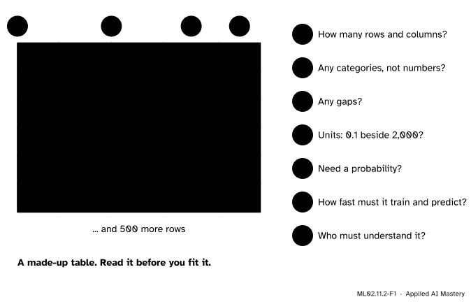
Seven questions, most of them answered by looking at the table. The clinic column holds names, not numbers. The area column has a gap, and its values are ten thousand times those beside it.

None of the seven needs a model fitted. Together they shorten the list of candidates, so the fair comparison of the next lesson has fewer models to compare.

Build it up

Take the questions one at a time, and say what each answer means for the families of Lesson 1.

Step 1. Rows and columns. With few rows, strong assumptions pay: linear models and naive Bayes learn from little data (ML02.6.4). With many rows, flexible models can show their worth, but their costs grow: \(k\)-NN compares each new row with every stored row, and an exact kernel method stores an \(n \times n\) matrix (ML02.8.4).

Step 2. Categories. A column such as “clinic” holds names. Boosted trees can split on a category directly (HistGradientBoosting with categorical_features, ML02.5). Linear models, \(k\)-NN and SVMs need it turned into numbers first, and one-hot encoding a column with thousands of levels makes thousands of features.

Step 3. Gaps. scikit-learn’s trees, forests and histogram boosting accept missing values (NaN) and learn which way to send them. Linear models, \(k\)-NN, SVMs and naive Bayes refuse them, so an imputer must fill the gaps, inside the pipeline.

Step 4. Units. A distance or a penalty adds features together, so the units matter. A tree asks one feature at a time whether it is above a threshold, so they do not.

ML02.11.2-F2

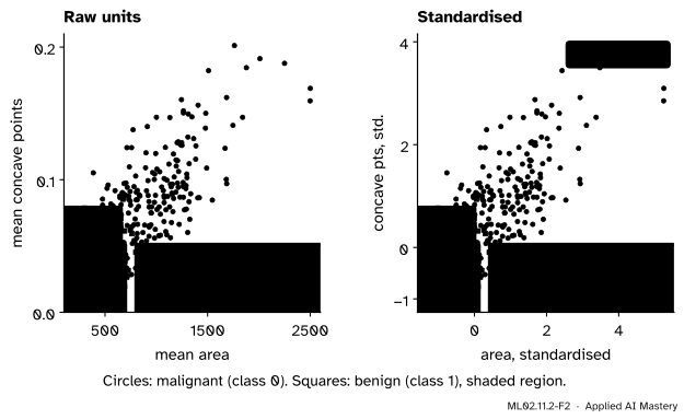
A tree grown on raw units and on standardised units. The rectangles are the same; only the numbers on the axes differ.

Step 5. Probabilities. If a decision needs a probability, prefer a model that gives a sound one. Logistic regression’s are usually reasonable. A small tree gives one value per leaf. Naive Bayes pushes probabilities to 0 and 1 when features are correlated (ML02.6.4). An SVM gives none without an extra step (ML02.7.4).

Step 6. Speed. Training once a night and predicting a million times a day are different problems. Linear models, trees and naive Bayes predict in a handful of operations. \(k\)-NN must search its stored rows for every prediction.

Step 7. Explanation. A linear model’s weights and a small tree can be read by a person. An ensemble of hundreds of trees cannot, and needs the tools of ML04.9.

Step 8. The evidence for tree ensembles. Grinsztajn, Oyallon and Varoquaux compared tuned tree ensembles with tuned deep networks on 45 tables. The trees came out ahead, and the authors traced it to the biases of Lesson 1: trees are robust to uninformative features, follow the orientation of the columns, and can learn irregular functions.

ML02.11.2-F6

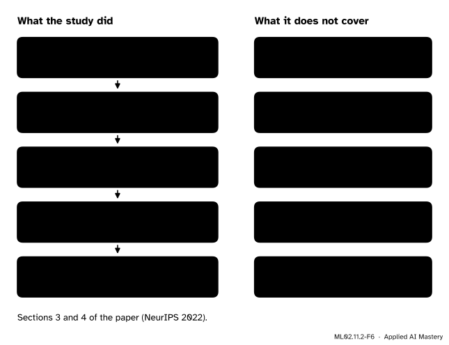
The benchmark’s path, and what it filtered out on the way. The finding holds for the tables on the left, not automatically for yours.

Read the right-hand column carefully. A table was dropped as “too easy” when a default linear model scored within 5 percent of both a default boosted-tree model and a default deep network. So the study says nothing about tables where a linear model is good enough, and Lesson 4 meets such a table. The evidence makes tree ensembles a strong default, never a replacement for a baseline and a fair comparison.

The formal statement

Two results explain Step 4.

Result 1: a tree does not change when a feature is standardised. Let \(g\) be any strictly increasing function, and replace feature \(j\) by \(g(x_j)\). For every threshold \(s\),

\[ x_j \le s \iff g(x_j) \le g(s), \]

because a strictly increasing function keeps order in both directions. So each split of the training rows that the tree could make before, it can make after, and no new ones appear. Each candidate split sends the same rows left and right, so it has the same impurity, and the greedy grower (ML02.1.3) makes the same choices. The tree cuts the training rows into exactly the same leaves.

New rows need one more step. The grower puts each threshold halfway between two neighbouring values \(a < b\). For standardising, \(g(x) = {(x - m)/s_j}\) with \(s_j > 0\), and halfway survives:

\[ \begin{aligned} \frac{g(a) + g(b)}{2} &= \frac{(a + b)/2 - m}{s_j} \\ &= g\Big(\frac{a + b}{2}\Big). \end{aligned} \]

So a standardised tree gives every new row the same prediction too. For a curved \(g\) such as a logarithm the midpoint can move, and a new row that falls between two training values may land differently.

Result 2: \(k\)-NN changes when a feature is rescaled. Multiply feature \(j\) by \(c > 0\). Its term in the squared distance becomes

\[ (c\,x_j - c\,z_j)^2 = c^2 (x_j - z_j)^2 , \]

so its weight in every distance is multiplied by \(c^2\). A feature measured in large units dominates, whatever its value for prediction. Standardising divides each feature by its standard deviation \(s_j\), so every feature enters on the same footing. The same holds for an RBF kernel, which depends on \(\norm{\vect{x} - \vect{z}}^2\), and for any penalty on the size of the weights.

ML02.11.2-F5

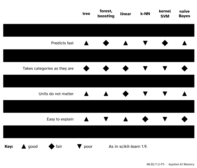
The checklist as a scorecard, for the scikit-learn estimators of this course. No column is green from top to bottom: every family pays somewhere.

The ratings summarise the earlier modules, not a theorem. Hastie, Tibshirani and Friedman publish a similar table (ESL Table 10.1) and reach the same verdict on trees: fast, unchanged by monotone transformations, resistant to irrelevant inputs, but seldom the most accurate alone.

Naive Bayes earns its mark for units because each feature’s Gaussian is fitted on that feature’s own scale. One small exception: scikit-learn’s GaussianNB adds a tiny multiple of the largest variance to every variance (var_smoothing), so when spreads differ by a factor of 200,000, as in the cancer table, standardising still changes about 1 percent of its predictions.

Worked example

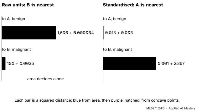
Units decide the nearest neighbour. Three patients, described by mean area and mean concave points. The standard deviations over all 569 patients are about \(352\) and \(0.039\).

Patient	area	concave points	diagnosis
new	\(600\)	\(0.030\)	?
A	\(640\)	\(0.032\)	benign
B	\(590\)	\(0.090\)	malignant

ML02.11.2-F3

The same two distances before and after standardising. In raw units the concave points cannot be seen; once each feature is divided by its spread, they decide.

Raw units. The squared distance to A is

\[ \begin{aligned} &(600 - 640)^2 + (0.030 - 0.032)^2 \\ &\quad= 1600 + 0.000004 . \end{aligned} \]

To B it is \({(600 - 590)^2} + {(0.030 - 0.090)^2} = {100 + 0.0036}\). B is nearer, so 1-NN calls the new tumour malignant, on the strength of a gap of 10 in area against one of 40.

Standardised. Divide each difference by its feature’s spread first. To A:

\[ \begin{aligned} &\Big(\frac{40}{352}\Big)^2 + \Big(\frac{0.002}{0.039}\Big)^2 \\ &\quad= 0.0129 + 0.0026 = 0.0155 . \end{aligned} \]

To B:

\[ \begin{aligned} &\Big(\frac{10}{352}\Big)^2 + \Big(\frac{0.060}{0.039}\Big)^2 \\ &\quad= 0.0008 + 2.3669 = 2.3677 . \end{aligned} \]

Now A is nearer by a wide margin, and the prediction is benign. The difference in concave points, \(0.060\), is one and a half standard deviations, and in raw units it was invisible.

Code

First the checklist, from scratch, on the real table.

import numpy as np
from sklearn.datasets import load_breast_cancer

data = load_breast_cancer()
X, y, names = data.data, data.target, data.feature_names

def profile(X):
    """The questions a table answers before any model is fitted."""
    spread = X.std(axis=0)
    return {"rows": X.shape[0], "features": X.shape[1],
            "all numeric": bool(np.issubdtype(X.dtype, np.number)),
            "missing cells": int(np.isnan(X).sum()),
            "widest spread": (str(names[spread.argmax()]), round(float(spread.max()), 1)),
            "narrowest spread": (str(names[spread.argmin()]), round(float(spread.min()), 4)),
            "ratio": round(float(spread.max() / spread.min()))}

for key, value in profile(X).items():
    print(f"{key:16} {value}")
print("classes (malignant, benign):", np.bincount(y))

rows             569
features         30
all numeric      True
missing cells    0
widest spread    ('worst area', 568.9)
narrowest spread ('fractal dimension error', 0.0026)
ratio            215171
classes (malignant, benign): [212 357]

Spreads differ by a factor of about 200,000, so Step 4 matters here. Score three models on raw and on standardised features, with the same five folds.

from sklearn.model_selection import StratifiedKFold, cross_val_score
from sklearn.neighbors import KNeighborsClassifier
from sklearn.pipeline import make_pipeline
from sklearn.preprocessing import StandardScaler
from sklearn.svm import SVC
from sklearn.tree import DecisionTreeClassifier

folds = StratifiedKFold(5, shuffle=True, random_state=0)
scores = {}
for name, model in [("k-NN", KNeighborsClassifier()), ("SVM, RBF", SVC()),
                    ("tree", DecisionTreeClassifier(random_state=0))]:
    raw = cross_val_score(model, X, y, cv=folds).mean()
    std = cross_val_score(make_pipeline(StandardScaler(), model), X, y, cv=folds).mean()
    scores[name] = (raw, std)
    print(f"{name:9} raw {raw:.3f}   standardised {std:.3f}")

k-NN      raw 0.932   standardised 0.965
SVM, RBF  raw 0.921   standardised 0.977
tree      raw 0.926   standardised 0.926

Standardising lifts \(k\)-NN from \(0.932\) to \(0.965\) and the RBF SVM from \(0.921\) to \(0.977\). The tree scores \(0.926\) both times, to the last digit, as Result 1 says. Check Result 1 directly, and with a logarithm as the increasing function:

from sklearn.model_selection import train_test_split

X_train, X_test, y_train, y_test = train_test_split(X, y, test_size=0.3, random_state=0, stratify=y)
scaler = StandardScaler().fit(X_train)
for label, g in [("standardise", scaler.transform), ("log(1 + x)", np.log1p)]:
    a = DecisionTreeClassifier(max_depth=3, random_state=0).fit(X_train, y_train)
    b = DecisionTreeClassifier(max_depth=3, random_state=0).fit(g(X_train), y_train)
    same_leaves = np.array_equal(a.apply(X_train), b.apply(g(X_train)))
    changed = int((a.predict(X_test) != b.predict(g(X_test))).sum())
    print(f"{label:12} same leaves for every training row: {same_leaves};  test predictions changed: {changed}")

standardise  same leaves for every training row: True;  test predictions changed: 0
log(1 + x)   same leaves for every training row: True;  test predictions changed: 0

The worked example, from scratch:

new, A, B = np.array([600, 0.030]), np.array([640, 0.032]), np.array([590, 0.090])
spread = np.array([352, 0.039])
for label, scale in [("raw", np.ones(2)), ("standardised", spread)]:
    dA, dB = np.sum(((new - A) / scale) ** 2), np.sum(((new - B) / scale) ** 2)
    print(f"{label:12} squared distance to A {dA:.4f}, to B {dB:.4f}: nearest is {'A' if dA < dB else 'B'}")
print("real spreads:", {str(names[j]): float(f"{X[:, j].std():.3g}") for j in (3, 7)})

raw          squared distance to A 1600.0000, to B 100.0036: nearest is B
standardised squared distance to A 0.0155, to B 2.3677: nearest is A
real spreads: {'mean area': 352.0, 'mean concave points': 0.0388}

Step 3, gaps. Blank out a random 10 percent of the cells.

from sklearn.ensemble import HistGradientBoostingClassifier, RandomForestClassifier
from sklearn.impute import SimpleImputer
from sklearn.linear_model import LogisticRegression

rng = np.random.default_rng(0)
X_gaps = X.copy()
X_gaps[rng.random(X.shape) < 0.1] = np.nan
print("cells missing:", round(float(np.isnan(X_gaps).mean()), 3), "  complete rows:", int((~np.isnan(X_gaps).any(axis=1)).sum()))
try:
    LogisticRegression().fit(X_gaps, y)
except ValueError:
    print("LogisticRegression refuses NaN")
RandomForestClassifier(n_estimators=10, random_state=0).fit(X_gaps, y)        # accepted
native = cross_val_score(HistGradientBoostingClassifier(random_state=0), X_gaps, y, cv=folds).mean()
imputed = cross_val_score(make_pipeline(SimpleImputer(strategy="median"), StandardScaler(), LogisticRegression()),
                          X_gaps, y, cv=folds).mean()
print(f"histogram boosting, gaps as they are: {native:.3f};  median imputation + logistic: {imputed:.3f}")

cells missing: 0.102   complete rows: 21
LogisticRegression refuses NaN
histogram boosting, gaps as they are: 0.963;  median imputation + logistic: 0.967

Only 21 of 569 rows are complete, so dropping incomplete rows is not an option. Either route works; what matters is that the imputer sits inside the pipeline, so it learns its medians from the training folds only (ML01.10.2).

Step 5, probabilities, on the 171 test patients:

from sklearn.naive_bayes import GaussianNB

tree3 = DecisionTreeClassifier(max_depth=3, random_state=0).fit(X_train, y_train)
logistic = make_pipeline(StandardScaler(), LogisticRegression()).fit(X_train, y_train)
p_tree, p_log = tree3.predict_proba(X_test)[:, 1], logistic.predict_proba(X_test)[:, 1]
p_nb = GaussianNB().fit(X_train, y_train).predict_proba(X_test)[:, 1]
print("different probabilities: tree", len(np.unique(p_tree)), "  logistic", len(np.unique(p_log.round(6))))
extreme = lambda p: np.mean(np.abs(p - 0.5) > 0.499)
print(f"share beyond 0.999 or below 0.001: naive Bayes {extreme(p_nb):.2f}, logistic {extreme(p_log):.2f}")

different probabilities: tree 6   logistic 149
share beyond 0.999 or below 0.001: naive Bayes 0.93, logistic 0.48

The depth-3 tree can only say one of six numbers. Naive Bayes is certain about 93 percent of the patients, though its accuracy does not justify that certainty. How to check and repair probabilities is ML04.7.

Explore

This module’s interactive, the model line-up, is in lesson 1. Its \(k\)-NN and logistic regression standardise the features inside the fit, as Step 4 asks, and its tree does not need to. Choose Rings and slide the training set down to 20 points: naive Bayes, whose strong assumption is Step 1’s advice for few rows, often still finds the circle. On a typical sample it scores above 0.8, while \(k\)-NN, with only six neighbours to vote, falls to about 0.7. Press New sample a few times: with so few points every score jumps.

Pitfalls

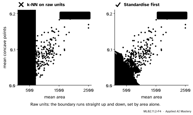
ML02.11.2-F4

Wrong beside right, on two features. In raw units the neighbours are chosen by area alone and the boundary runs straight up the page. Standardised, the concave points count too.

“I’ll standardise every feature for every model, to be safe.”

For a tree it is harmless and pointless (Result 1). For \(k\)-NN, SVMs and penalised linear models it is essential. But it must happen inside the pipeline: a scaler fitted on all the rows has seen the held-out ones (ML01.10.2).

“The benchmark proved boosting beats everything on tables, so I can skip the baseline.”

The benchmark removed every table on which a default linear model came within 5 percent of two strong default models, and it did not include linear models, \(k\)-NN or SVMs as contenders. It shows that tuned tree ensembles beat tuned deep networks on medium tables that need more than a straight line. Your table may be one of the easy ones. Fit the baseline.

“Accuracy is the only line of the checklist that matters.”

A model that must give a probability, explain itself to a regulator or answer in a millisecond can lose on accuracy and still be the right choice. Decide which lines matter before you look at any score, so that the scores cannot talk you out of them.

Check yourself

Recall

1. Name four of the seven checklist questions.

Show answer

Any four of: how many rows and columns; any categorical columns; any missing values; do the units differ; is a probability needed; how fast must it train and predict; who must understand it.

2. Why does standardising not change a decision tree?

Show answer

A split asks whether \(x_j \le s\), and a strictly increasing change of units keeps that answer for every row. Standardising also keeps midpoints, so the same splits, thresholds and leaves result.

3. What happens to a feature’s weight in a \(k\)-NN distance when it is measured in units ten times smaller?

Show answer

Its values grow tenfold, so its term in the squared distance is multiplied by \(100\).

4. Which scikit-learn models accept NaN as it is, and what must the others have?

Show answer

Trees, forests and histogram gradient boosting. The others need an imputer, placed inside the pipeline.

5. Which tables did the Grinsztajn, Oyallon and Varoquaux benchmark leave out?

Show answer

Among others: tables a default linear model already fits nearly as well as the best (“too easy”), rows with missing values, categories with over 20 levels, and tables under 3,000 rows.

Exercises

1. ★ A feature is recorded in metres and you change it to millimetres. By what factor does its term in a squared distance change? What happens to a tree’s predictions?

Show solution

Each value is multiplied by \(c = 1000\), so by Result 2 its term is multiplied by \(c^2 = 1{,}000{,}000\). The tree is unchanged: multiplying by \(1000\) is strictly increasing and keeps midpoints, so by Result 1 every split, leaf and prediction stays the same.

2. ★★ For each table, name one family you would put on the shortlist and one you would leave off, with a reason from the checklist. (a) 300 rows, 8 numeric features, the doctor must see why. (b) 2 million rows, 40 features, a fifth of the cells missing, predictions needed in a millisecond. (c) 5,000 rows, a “postcode” column with 3,000 values.

Show solution

(a) On: logistic regression or a small tree, which can be read and suit few rows. Off: a large boosted ensemble, which cannot be read without extra tools.

(b) On: histogram gradient boosting, which handles gaps natively, trains on many rows and predicts fast. Off: \(k\)-NN, which would search millions of stored rows for each prediction and needs every gap filled.

(c) On: boosted trees with native categorical splits, or target encoding with care (ML02.5.3). Off: one-hot encoding into a linear model or \(k\)-NN, which turns one column into 3,000 sparse ones.

3. ★★★ Result 1 says a strictly increasing \(g\) leaves a tree’s training leaves unchanged. Show with a three-point example that the prediction for a new row can change when \(g(x) = x^2\) on positive values.

Show solution

Take training values \(x = 1\) (class 0) and \(x = 3\) (class 1). The tree splits halfway, at \(x \le 2\). After \(g(x) = x^2\) the training values are \(1\) and \(9\), and the split is at \(x^2 \le 5\), that is \(x \le \sqrt{5} \approx 2.24\). A new row with \(x = 2.1\) goes right (class 1) in the first tree, since \(2.1 > 2\), and left (class 0) in the second, since \(2.1^2 = 4.41 \le 5\). The training rows are split the same way; only the threshold between them moved.

Summary card

Read the table before you fit it: its size, types, gaps, units and uses shorten the list.

The anchor figure again: a made-up table with a category column, a missing cell and columns in very different units, beside the seven checklist questions. — ML02.11.2-F1
Seven questions, no model fitted.

Trees: unchanged by any strictly increasing change of units; standardising keeps every prediction.
Distances: rescaling feature \(j\) by \(c\) multiplies its term by \(c^2\); standardise for \(k\)-NN, SVMs, penalties.
Gaps: trees, forests, histogram boosting accept NaN; others need an imputer in the pipeline.
Evidence: tree ensembles beat deep nets on medium tables that are not “too easy”; always fit a baseline.

Sources and next steps

Sources. Each was opened and checked against this lesson on 15 November 2026.

Trevor Hastie, Robert Tibshirani and Jerome Friedman, The Elements of Statistical Learning, 2nd edition, corrected 12th printing. Section 10.7 and Table 10.1 (page 351) rate neural nets, SVMs, trees, MARS and \(k\)-NN on mixed data, missing values, monotone transformations, scalability, irrelevant inputs, interpretability and predictive power; the text calls trees invariant under strictly monotone transformations and resistant to irrelevant inputs, but seldom the most accurate.
Léo Grinsztajn, Edouard Oyallon and Gaël Varoquaux, Why do tree-based models still outperform deep learning on typical tabular data?, NeurIPS 2022 Datasets and Benchmarks Track. Section 3.1: the selection criteria, including “not too easy” (a default linear model within 5 percent of both a ResNet and HistGradientBoosting) and at least 3,000 rows. Section 3.2: training sets cut to 10,000 rows, rows with missing values removed, categories with more than 20 levels removed. Section 4: the tree models (random forest, gradient boosting, XGBoost) against MLP, ResNet, FT-Transformer and SAINT.
scikit-learn 1.9 user guide. Section 1.10.8: decision trees accept missing values; the same page says the implementation does not support categorical variables. Section 1.11.1.1: histogram gradient boosting has built-in support for missing values (1.11.1.1.2) and categorical features through categorical_features (1.11.1.1.4).

Next. ML02.11.3 A fair comparison takes the shortlist and decides between its members, with error bars honest enough to say when it cannot.

This lesson unlocks

ML02.11.3 A fair comparison

Your progress is saved in this browser only. No account, no tracking.