import numpy as np
from sklearn.compose import TransformedTargetRegressor
from sklearn.datasets import load_diabetes
from sklearn.dummy import DummyRegressor
from sklearn.ensemble import HistGradientBoostingRegressor, RandomForestRegressor
from sklearn.kernel_ridge import KernelRidge
from sklearn.linear_model import Lasso, LinearRegression
from sklearn.model_selection import GridSearchCV, KFold, RepeatedKFold, cross_validate, train_test_split
from sklearn.pipeline import make_pipeline
from sklearn.preprocessing import StandardScaler
from sklearn.svm import SVR
from sklearn.tree import DecisionTreeRegressor

data = load_diabetes(scaled=False)
X_work, X_test, y_work, y_test = train_test_split(data.data, data.target, test_size=89, random_state=10)
inner, mae = KFold(5, shuffle=True, random_state=1), "neg_mean_absolute_error"
tuned = lambda model, grid: GridSearchCV(model, grid, cv=inner, scoring=mae)
candidates = {
    "baseline": DummyRegressor(strategy="median"),
    "lasso": make_pipeline(StandardScaler(), Lasso(alpha=5)),
    "linear": LinearRegression(),
    "tree": tuned(DecisionTreeRegressor(random_state=0), {"ccp_alpha": [25, 50, 100, 200, 400, 800]}),
    "forest": RandomForestRegressor(n_estimators=200, min_samples_leaf=5, max_features=1 / 3, random_state=0),
    "boosting": HistGradientBoostingRegressor(learning_rate=0.05, max_iter=100, max_depth=3, random_state=0),
    "svr": tuned(make_pipeline(StandardScaler(), SVR()), {"svr__C": [10, 30, 100, 300]}),
    "krr": TransformedTargetRegressor(tuned(make_pipeline(StandardScaler(), KernelRidge(kernel="rbf")),
                                            {"kernelridge__alpha": [0.3, 1, 3], "kernelridge__gamma": [0.003, 0.01, 0.03]}),
                                      transformer=StandardScaler()),
}
folds = RepeatedKFold(n_splits=5, n_repeats=3, random_state=0)
scores = {name: -cross_validate(model, X_work, y_work, cv=folds, scoring=mae)["test_score"]
for name, model in candidates.items()}Case study: the diabetes project revisited
The diabetes project of ML01.10 rerun with every model of this course: a pruned tree, a random forest, gradient boosting, SVR and kernel ridge against the linear models, on the same patients and the same repeated folds, ending in a choice and a one-page report.
Before this lesson: ML02.11.3 A fair comparison ML01.10.4 Analyse errors and write it up
What you will be able to do
- Run a fair comparison of eight candidates on a real table, with every tuning step nested inside the outer folds.
- Read a results table with corrected standard errors and apply the one-standard-error rule with a simplicity order fixed in advance.
- Explain from each model’s inductive bias why tree ensembles do not win on this table.
- Write the five-part report and say honestly what the test set can and cannot still tell you.
The question
ML01.10 predicted how far diabetes would progress in a year from ten measurements at a first visit, and chose the lasso: a cross-validated error of \(46.3\) points. Since then this course has built trees, forests, boosting, support vector regression and kernel ridge. Does any of them beat a straight line on this table? And if one scores a point lower, should the clinic switch?
From the last lesson
1. Write the corrected standard error for \(J\) differences from \(k\)-fold splits.
Show answer
\(\text{SE}_\text{corr} = s\sqrt{1/J + 1/(k-1)}\), with \(s\) the standard deviation of the differences.
2. Why is the best of 30 tuned scores too optimistic?
Show answer
It is the luckiest of 30 noisy estimates. Nested cross-validation, which scores the whole tuning procedure on folds it never saw, removes the bias.
Intuition
Same patients, same metric, same 89 patients locked away as in ML01.10. What changes is the line of candidates, and the folds: five folds repeated three times, with the corrected error bars of Lesson 3.
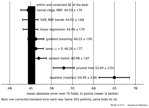
Every candidate on the same 15 folds. Six models crowd within three points of each other, far from the baseline. Only three sit inside the band of one corrected standard error of the best.
The picture answers the first question. The flexible models do not run away from the linear ones; kernel ridge is lowest, by \(0.6\) points, and its error bar is three times wider than that. The second question needs the rule.
Build it up
Step 1. The checklist (Lesson 2). 353 working rows and 10 numeric features, no gaps, one two-valued code (sex), and units that differ: age runs from 19 to 79 years, s5 from 3.3 to 6.1. Small and clean: every family is allowed, and those that measure distance need standardising.
Step 2. The candidates. The two linear models of ML01.10 and five new ones, each a pipeline:
- a pruned tree, its
ccp_alphachosen by inner cross-validation (ML02.1.4); - a random forest of 200 trees, a third of the features per split, at least five patients per leaf (ML02.2.3);
- gradient boosting with
HistGradientBoostingRegressor, 100 trees of depth 3 at learning rate \(0.05\) (ML02.4, ML02.5); - SVR with an RBF kernel on standardised features, \(C\) chosen by inner cross-validation (ML02.7.4);
- kernel ridge with an RBF kernel, its \(\lambda\) and \(\gamma\) chosen by inner cross-validation, with the target standardised because kernel ridge has no intercept (ML02.8.4).
Step 3. Tuning goes inside. Each GridSearchCV is itself the model. On every outer split it tunes on the training rows only, so the outer folds score the whole procedure, tuning included: nested cross-validation, the remedy of Lesson 3.
Step 4. Look at the shapes. Why might boosting fail to beat a line? Hold nine measurements at typical values and vary body mass index.
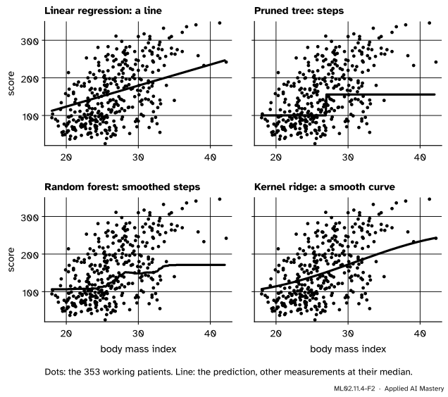
Four inductive biases on one feature. The tree and the forest can only step, and are flat beyond the data’s edges; kernel ridge bends but chooses to stay close to a line.
The trend is close to straight, and 353 noisy patients cannot reveal much more. A model built from steps must approximate a line with stairs, and pays for it (Lesson 1). Kernel ridge can bend, but the data give it no reason to.
Step 5. The rule, fixed before looking. Take the lowest mean error. Its corrected standard error sets a limit. Among candidates inside the limit, take the simplest, in this order fixed in advance: lasso (5 weights), pruned tree (5 leaves), linear regression (10 weights), then the kernel methods (353 coefficients each), then the ensembles (hundreds of trees).
The formal statement
This is the one-standard-error rule of ML01.10.3 with one change: the error bar is corrected for repeated folds. The factor is \(\sqrt{1/15 + 1/4} = \sqrt{0.3167} = 0.563\), against \(1/\sqrt{15} = 0.258\) uncorrected.
Pairs, as a check. The rule compares each score with the best one’s error bar. Lesson 3’s paired comparison asks a sharper question of each candidate: is it decidedly worse than the best, by more than two corrected standard errors of the paired differences?
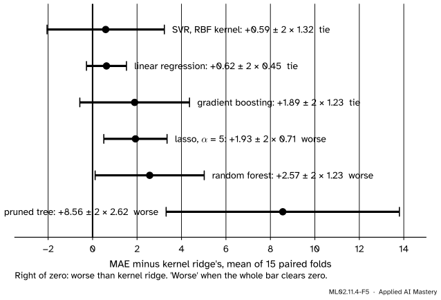
Each candidate minus kernel ridge, fold by fold. SVR, linear regression and boosting cannot be told from it; the lasso, the forest and the tree are decidedly worse.
Both views agree on what matters: linear regression is a tie with the best, and the lasso is not. Pairing narrows the linear model’s bar to \(\pm 2 \times 0.45\), because a fold that is hard for kernel ridge is hard for a straight line too.
Worked example
The choice, by hand, from the table of results.

Four steps from the results table to a choice.
Step 1. The lowest mean is kernel ridge’s, \(44.33\), with fold standard deviation \(3.09\). Its error bar is \(3.09 \times 0.563 = 1.74\).
Step 2. The limit is \({44.33 + 1.74} = 46.07\).
Step 3. Inside: kernel ridge \(44.33\), SVR \(44.92\), linear regression \(44.96\). Outside, if only just: boosting \(46.23\) and the lasso \(46.26\); then the forest \(46.90\) and the tree \(52.89\).
Step 4. Of the three inside, linear regression comes first in the simplicity order. Linear regression on all ten measurements goes forward.
Check with pairs. Linear regression minus kernel ridge, over the 15 folds, has mean \(0.62\) and corrected standard error \(0.45\): \(1.4\) errors from zero, a tie. The lasso minus kernel ridge is \({1.93 \pm 0.71}\): \(2.7\) errors, decidedly worse.
So the choice differs from ML01.10’s. There, five folds gave the lasso \({1.13 \pm 1.13}\) behind linear regression, a tie, and simplicity chose the lasso. Fifteen folds put it \(1.30\) behind, and the limit now falls between them. Nothing was wrong then; more folds narrowed the error bar enough to see a gap that five could not.
Code
The protocol, exactly as stated. Every tuned candidate is a GridSearchCV, so its tuning runs inside each outer split.
From scratch, the error bars and the rule.
def corrected_se(values, k=5):
    return values.std(ddof=1) * np.sqrt(1 / len(values) + 1 / (k - 1))

simplest_first = ["lasso", "tree", "linear", "svr", "krr", "forest", "boosting"]
table = sorted(scores, key=lambda name: scores[name].mean())
for name in table:
    print(f"{name:9} {scores[name].mean():6.2f} +/- {corrected_se(scores[name]):.2f}")

best = table[0]
limit = scores[best].mean() + corrected_se(scores[best])
inside = [name for name in simplest_first if scores[name].mean() <= limit]
print(f"best: {best}; limit {limit:.2f}; inside, simplest first: {inside}; chosen: {inside[0]}")
for name in ("linear", "lasso", "boosting"):
    d = scores[name] - scores[best]
    print(f"{name:9} minus {best}: {d.mean():+.2f} +/- {corrected_se(d):.2f}  ({d.mean() / corrected_se(d):.1f} SE)")
krr 44.33 +/- 1.74
svr 44.92 +/- 1.88
linear 44.96 +/- 1.79
boosting 46.23 +/- 1.96
lasso 46.26 +/- 1.77
forest 46.90 +/- 1.87
tree 52.89 +/- 2.54
baseline 64.96 +/- 3.66
best: krr; limit 46.07; inside, simplest first: ['linear', 'svr', 'krr']; chosen: linear
linear minus krr: +0.62 +/- 0.45 (1.4 SE)
lasso minus krr: +1.93 +/- 0.71 (2.7 SE)
boosting minus krr: +1.89 +/- 1.23 (1.5 SE)What the tuned models chose, fitted on all 353 working rows, and how much each has to show for itself:
fitted = {name: candidates[name].fit(X_work, y_work) for name in ("tree", "svr", "krr", "linear")}
print("tree:", fitted["tree"].best_params_, "leaves:", fitted["tree"].best_estimator_.get_n_leaves())
print("SVR:", fitted["svr"].best_params_, "support vectors:", len(fitted["svr"].best_estimator_[-1].support_))
print("kernel ridge:", fitted["krr"].regressor_.best_params_)
weights = {name: float(w) for name, w in zip(data.feature_names, fitted["linear"].coef_.round(2))}
print("linear regression, points per unit of each measurement:", weights)
tree: {'ccp_alpha': 200} leaves: 5
SVR: {'svr__C': 300} support vectors: 353
kernel ridge: {'kernelridge__alpha': 0.3, 'kernelridge__gamma': 0.03}
linear regression, points per unit of each measurement: {'age': -0.01, 'sex': -21.51, 'bmi': 5.58, 'bp': 1.13, 's1': -1.0, 's2': 0.64, 's3': 0.3, 's4': 8.05, 's5': 64.2, 's6': 0.17}The pruned tree keeps 5 leaves; the SVR keeps every one of the 353 patients as a support vector, so it is no sparser than kernel ridge. The linear weights are in points of the score per unit: \(5.58\) per unit of body mass index, \(64.2\) per unit of s5, which scikit-learn describes as possibly the log of the serum triglycerides level.
The report
Explore
This module’s interactive, the model line-up, is in lesson 1. Pick the Diagonal line and slide the training-set size up and down: with a straight boundary and little data the linear model leads and the tree trails, the same story as this lesson’s table.
Pitfalls
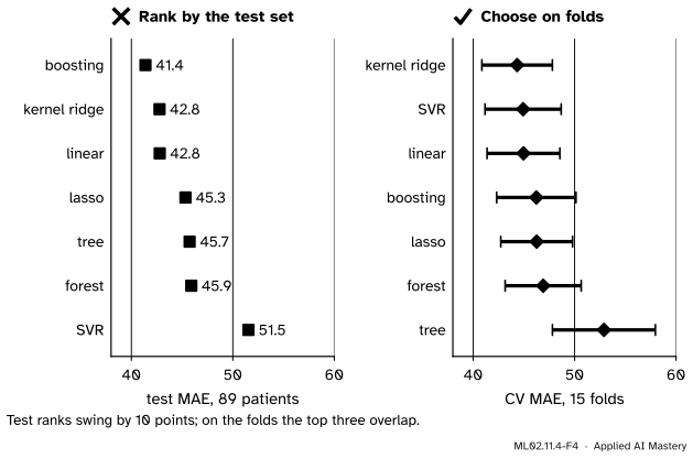
Wrong beside right. Ranked by 89 test patients, boosting is first and SVR last, ten points apart; on 15 folds they are \(1.3\) points apart. The test set is too small to choose with, and every look at it spends its honesty.
“Boosting scored 41.4 on the test set, the best of all. Switch to boosting.”
That number was found by opening the test set for every candidate, which is shown here once, as a warning. Eighty-nine patients give each test score a standard error of \(3.5\) to \(4.3\), so the test ranking is mostly noise: SVR, a tie for first on the folds, comes last. Choose on the folds; open the test set once, for the chosen model.
“Kernel ridge has the lowest error, so it is the best model.”
It is lowest by \(0.62\) points, with a corrected standard error of \(0.45\) for the gap: not decided. Between models the data cannot separate, choose the one you can explain, check and maintain: here, ten weights.
“Tree ensembles win on tabular data, so something must be wrong with my setup.”
The benchmark of Lesson 2 removed tables like this one, where a linear model is about as good as the best. Small, nearly linear and noisy: here the straight line is the right inductive bias.
Check yourself
Recall
1. Why does putting GridSearchCV inside cross_validate make the comparison fair to the tuned models?
Show answer
The tuning is redone on the training rows of every outer split, so each outer fold scores the whole procedure, tuning included: nested cross-validation. The tuned models are not flattered.
2. State the choice rule used in this lesson.
Show answer
Keep every candidate whose mean error is at most the best mean plus the best’s corrected standard error, and choose the simplest of them in an order fixed in advance.
3. Which candidates were inside the limit, and which was chosen?
Show answer
Kernel ridge (\(44.33\)), SVR (\(44.92\)) and linear regression (\(44.96\)), inside \(46.07\). Linear regression, the simplest of the three.
4. Why do the forest and the tree flatten out at the extremes of body mass index?
Show answer
They predict averages of training targets in boxes, so beyond the last split the prediction is constant. They cannot extrapolate a trend.
5. Why is the test score of linear regression no longer quoted as an untouched estimate?
Show answer
The test set was opened in ML01.10.4, and the linear model’s test score was seen there. A score that has been seen before a choice can no longer stand as an independent check of that choice.
Exercises
1. ★ A ninth candidate scores \(45.80\) with fold standard deviation \(3.20\) over the same 15 folds. Is it inside the limit? Would the choice change?
Show solution
The limit is set by the best, \(44.33 + 1.74 = 46.07\), and \(45.80 \le 46.07\), so it is inside. The choice changes only if it is simpler than linear regression in the fixed order; if it comes after linear regression, linear regression still goes forward.
2. ★★ With five folds and no repeats, kernel ridge’s fold standard deviation is \(3.09\) as before. Compute the corrected and the uncorrected standard errors, then the limit. Is the lasso (\(46.26\)) inside either?
Show solution
With \(J = 5\) and \(k = 5\), corrected: \(3.09\sqrt{1/5 + 1/4} = 3.09\sqrt{0.45} = 3.09 \times 0.671 = 2.07\), so the limit is \({44.33 + 2.07} = 46.40\) and the lasso is inside. Uncorrected: \(3.09/\sqrt{5} = 1.38\), limit \(45.71\), and the lasso is outside. Fewer folds mean a wider honest error bar, which lets more candidates tie.
3. ★★★ A colleague suggests choosing by the paired rule instead: keep every candidate whose mean difference from the best is less than two corrected standard errors of the paired differences. Using the figures of the lesson, which candidates are kept, and which is chosen? Explain why the two rules can disagree.
Show solution
From the paired figure: SVR (\(0.59/1.32 = 0.4\)), linear regression (\(0.62/0.45 = 1.4\)) and boosting (\(1.89/1.23 = 1.5\)) are within two errors of kernel ridge; the lasso (\(2.7\)), the forest (\(2.57/1.23 = 2.1\)) and the tree are not. Kept: kernel ridge, SVR, linear regression and boosting. The simplest is still linear regression. The rules can disagree because the one-standard-error rule compares a candidate’s mean with one standard error of the best’s own score, while the paired rule uses the spread of the differences, which is small when two models rise and fall together across folds (lasso and kernel ridge) and large when they do not (boosting and kernel ridge).
Summary card
On a small, nearly linear table, no model of the course decidedly beats a straight line, and the straight line goes forward.
Six models within three points.
- Protocol: same 15 folds for all; tuning nested inside; corrected SE \({s_\text{fold}\sqrt{1/15 + 1/4}}\).
- Result: kernel ridge \({44.33 \pm 1.74}\), SVR \(44.92\), linear \({44.96 \pm 1.79}\); limit \(46.07\).
- Choice: linear regression, the simplest inside the limit.
- Next: ML04 adds feature engineering, tuning, calibration and interpretation.
Sources and next steps
Sources. Each was opened and checked against this lesson on 15 November 2026.
- Bradley Efron, Trevor Hastie, Iain Johnstone and Robert Tibshirani, Least Angle Regression, Annals of Statistics 32 (2004). Section 1 and Table 1 describe the diabetes data: 442 patients, ten baseline variables (age, sex, body mass index, blood pressure and six serum measurements) and a measure of disease progression one year after baseline.
- Trevor Hastie, Robert Tibshirani and Jerome Friedman, The Elements of Statistical Learning, 2nd edition. Section 7.10.1 describes \(K\)-fold cross-validation and the one-standard-error rule: choose the most parsimonious model whose error is no more than one standard error above the best.
- scikit-learn 1.9 user guide. Section 1.3, Kernel ridge regression: ridge regression combined with the kernel trick, fitted in closed form. Section 1.4.2, Regression: support vector regression, whose cost ignores samples predicted close to their target, so the model depends only on the others (here, with the default \(\varepsilon\) of \(0.1\) points, all 353 count). Section 3.1:
cross_validate(3.1.1.1),RepeatedKFold(3.1.2.1.2), pipelines that learn preprocessing from the training folds only (3.1.1), and a linked example of nested against non-nested cross-validation.
Next. This is the last lesson of ML02. The course on model development and evaluation in practice takes the project further: engineering features (ML04.2), cross-validation designs and tuning done properly (ML04.4, ML04.5), probabilities you can trust (ML04.7) and explaining what a model has learned (ML04.9).
This lesson unlocks
ML04 Model Development and Evaluation in Practice
Your progress is saved in this browser only. No account, no tracking.