An average error hides who the model fails. This lesson breaks the chosen model’s errors down by group, shows why errors lean against the outcome even for a sound model, opens the test set exactly once, puts an interval on the result and writes the one-page report.
Make out-of-fold predictions and use them to study a model’s errors without touching the test set.
Break a mean absolute error down by group, with a standard error for each group.
Explain why the errors of a least-squares model are correlated with the target and not with the prediction.
Evaluate the final model once on the test set and give a 95 percent interval for its score.
Write a short report with five parts: question, data, method, result and limits.
In review. The maths and code on this page are checked by automated tests on every change, but an independent reader has not signed it off yet. Spot a mistake or a confusing step? Tell us.
The question
The model that goes forward has a cross-validated error of \(46.3\) points. That is one number for 353 patients. Is it \(46\) for everyone, or \(30\) for some and \(60\) for others? And when the clinic asks “how good will it be on next year’s patients?”, what is the one number you can honestly promise, and how sure are you of it?
From the last lesson
1. What does the one-standard-error rule choose?
Show answer
The simplest setting whose cross-validated score is no more than one standard error above the lowest score.
2. Linear regression scored \(45.14\) and the lasso \(46.27\). Why did the lasso go forward?
Show answer
The gap was \(1.13\) with a standard error of \(1.13\), so the two cannot be told apart, and the lasso is simpler: it uses five of the ten features.
Intuition
To study a model’s mistakes you need predictions for patients it has not seen. The test set is still locked. But cross-validation has already produced exactly that: each patient sat in one held-out fold, and was predicted by a model trained on the other four. Collect those 353 out-of-fold predictions and set each beside the truth.
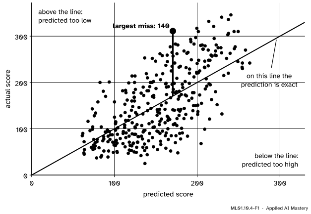
ML01.10.4-F1
Every working patient, predicted by a model that never saw them. The vertical distance from the line is the size of the error. The cloud is wide: a typical miss is 40 to 50 points.
The picture already says three things. The model has real skill, because the cloud slopes upwards. The predictions are bunched: they span about 200 points and the truth spans over 300. And single patients can be off by more than 100. The next steps put numbers on each.
Build it up
Step 1. Summarise the errors. As everywhere in this course, the error is the prediction minus the target, so a positive error means the model predicted too high. Half of the 353 errors are smaller in size than \(41.5\) points and a quarter are larger than \(66.5\). Twenty-six patients, 7 percent, are off by more than \(100\). The mean error is \(-0.1\): the model does not lean high or low overall.
Step 2. Ask for whom. Split the patients by something known at the first visit, and compute the MAE inside each group, with its standard error.
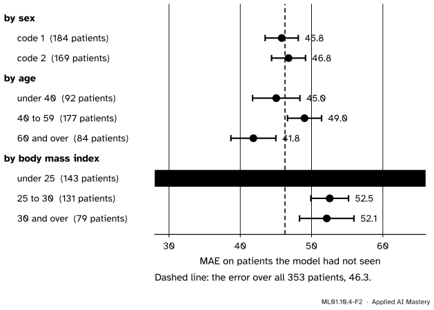
ML01.10.4-F2
The same error, group by group. Sex and age make little difference. Body mass index does: the error is \(37\) for patients under 25 and \(52\) above.
The two sex codes differ by one point, well inside their error bars. The age groups differ by a few points, about what their error bars allow. Body mass index is different. Patients with a BMI under 25 are predicted with an error of \(37.3\), and the rest with \(52.4\). The model is one model, but it is not equally reliable for everyone, and the report must say so.
Step 3. Read the worst cases. The largest error belongs to a patient predicted at \(171\) whose score was \(311\). None of that patient’s ten measurements is unusual: all lie within \(1.3\) standard deviations of the average. Some of what drives progression is simply not in the table, and no model built on these columns can know it.
Step 4. Freeze everything, then open the test set once. The pipeline, its \(\alpha\) and the metric are fixed. Fit the pipeline on all 353 working rows and predict the 89 test patients. This happens one time. If the number disappoints, it is still the number.
Step 5. Put an interval on it. The test MAE is a mean of 89 absolute errors, so it has a standard error, and about two standard errors either side make a 95 percent interval.
Step 6. Write it up. Five parts: the question, the data, the method, the result, the limits.
The formal statement
NoteDefinition: error, and error in a group
The error of a prediction is \(\closs{e_i} = {\cmodel{\hat{y}_i} - \ctruth{y_i}}\). For a group \(G\) of \(n_G\) patients, the group’s error and its standard error are
\[
\begin{aligned}
\text{MAE}_G &= \frac{1}{n_G}\sum_{i \in G} \abs{e_i}, \\[4pt]
\text{SE}_G &= \frac{\text{sd of the } \abs{e_i} \text{ in } G}{\sqrt{n_G}} .
\end{aligned}
\]
Result 1: the overall error is a weighted mean of the group errors. If the groups \(G_1, \dots, G_m\), of sizes \(n_1, \dots, n_m\), together hold every patient once, split the sum group by group:
An average of unequal numbers lies between them. So whenever groups differ, the overall MAE is too kind to one group and too harsh on another.
Result 2: an interval for a test score. The test MAE is the mean \(\bar{a}\) of \(n\) absolute errors with standard deviation \(s\). Its standard error is \(s/\sqrt{n}\) (ML01.2.3), and a 95 percent interval is
\[
\bar{a} \;\pm\; t \cdot \frac{s}{\sqrt{n}} ,
\]
where \(t\) is close to \(2\): it is \(1.99\) for \(n = 89\), the 97.5 percent point of Student’s \(t\) distribution with \(n - 1\) degrees of freedom. Intervals built this way cover the true value in about 95 of 100 repetitions.
Result 3: errors lean against the target, even for a sound model. Take a least-squares model with a bias, on its own training rows. ML01.4.3 showed that its errors satisfy the normal equations: they sum to zero, and so does their product with each feature,
because \(R^2 = {1 - \text{Var}(e)/\text{Var}(y)}\) (ML01.4.4). Unless the fit is perfect this is negative: the model predicts too high for low targets and too low for high ones. That is not a flaw to repair. It is what any honest prediction from incomplete information looks like. The lesson for error analysis: group by what is known when predicting, never by the outcome.
Go deeper: is the model really better for slim patients?
Its error is lower for them, \(37.3\) against \(52.4\). But their scores are also less spread out: always predicting their own median would score \(40.0\), against \(64.8\) for the others. So the model removes \({1 - 37.3/40.0} = 7\) percent of the error for patients with a BMI under 25, and \({1 - 52.4/64.8} = 19\) percent for the rest. In absolute terms it is more accurate for the first group. In terms of skill it does more for the second. A report should say which it means.
Worked example
Two groups by hand. Under 25: \(n = 143\), MAE \(37.3\), SE \(2.4\). BMI 25 and over: \(n = 210\), MAE \(52.4\), SE \(2.2\).
Result 1.\({(143 \times 37.3 + 210 \times 52.4)/353} = {(5334 + 11004)/353} = 46.3\), the overall MAE.
Is the gap real? It is \({52.4 - 37.3} = 15.1\). The two groups share no patient, so the squared standard errors add: \(\sqrt{2.4^2 + 2.2^2} = \sqrt{10.6} = 3.3\). The gap is more than four of its standard errors. It is real.
The test set, opened once. The 89 absolute errors have mean \(45.33\) and standard deviation \(33.54\).
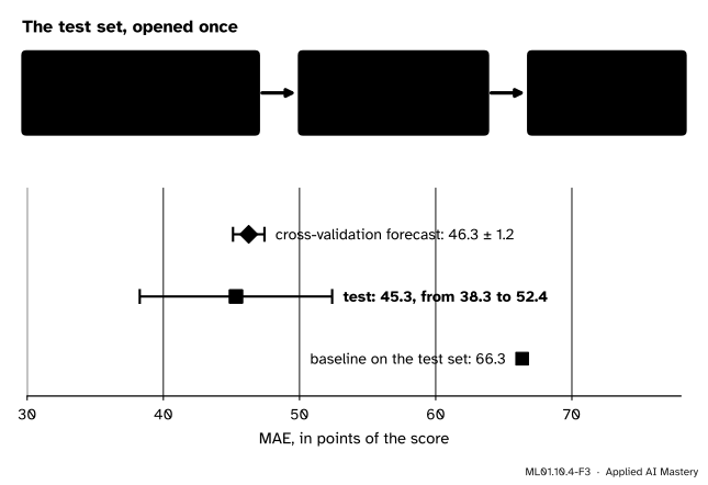
ML01.10.4-F3
From 89 errors to one score with an interval. The forecast from cross-validation sits well inside the interval, and the baseline far outside it.
Standard error.\(33.54/\sqrt{89} = 33.54/9.434 = 3.555\).
Interval.\({1.99 \times 3.555} = 7.07\), so the interval runs from \({45.33 - 7.07} = 38.3\) to \({45.33 + 7.07} = 52.4\).
Against the forecast. Cross-validation promised \({46.27 \pm 1.16}\). The test says \(45.33\). They agree.
Against the baseline. Always predicting the working median scores \(66.35\) on the same 89 patients. The model’s skill is \({1 - 45.33/66.35} = 0.32\).
Code
Out-of-fold predictions from scratch: one loop over the folds, filling in each held-out block.
import numpy as npfrom sklearn.datasets import load_diabetesfrom sklearn.linear_model import Lasso, LinearRegressionfrom sklearn.model_selection import KFold, cross_val_predict, train_test_splitfrom sklearn.pipeline import make_pipelinefrom sklearn.preprocessing import StandardScalerdata = load_diabetes(scaled=False)X_work, X_test, y_work, y_test = train_test_split(data.data, data.target, test_size=89, random_state=10)folds = np.array_split(np.arange(len(y_work)), 5)chosen = make_pipeline(StandardScaler(), Lasso(alpha=5)) # the pipeline that lesson 3 sent forwardpredicted = np.empty(len(y_work))for held in folds: train = np.setdiff1d(np.arange(len(y_work)), held) predicted[held] = chosen.fit(X_work[train], y_work[train]).predict(X_work[held])error = predicted - y_work # positive: the model predicted too highsize = np.abs(error)print(f"MAE {size.mean():.2f} RMSE {np.sqrt(np.mean(error **2)):.2f} mean error {error.mean():.2f}")print("quartiles of the error size:", np.percentile(size, [25, 50, 75]).round(1), " largest:", size.max().round(1))print("patients off by more than 100:", int((size >100).sum()))print("same as cross_val_predict:", np.allclose(predicted, cross_val_predict(chosen, X_work, y_work, cv=KFold(n_splits=5))))
MAE 46.27   RMSE 55.80   mean error -0.10
quartiles of the error size: [20.5 41.5 66.5]   largest: 140.4
patients off by more than 100: 26
same as cross_val_predict: True
The RMSE, \(55.8\), is about a fifth above the MAE, \(46.27\): by lesson 1’s Result 2 the error sizes are uneven, but no single miss dominates. Now the groups.
def by_group(masks):"""MAE, standard error and mean error inside each group."""for label, mask in masks.items(): s = size[mask]print(f"{label:16} n {mask.sum():3d} MAE {s.mean():5.1f} +/- {s.std(ddof=1) / np.sqrt(mask.sum()):.1f}"f" mean error {error[mask].mean():6.1f}")age, sex, bmi = X_work[:, 0], X_work[:, 1], X_work[:, 2]by_group({"sex code 1": sex ==1, "sex code 2": sex ==2})by_group({"age under 40": age <40, "age 40 to 59": (age >=40) & (age <60), "age 60 and over": age >=60})by_group({"BMI under 25": bmi <25, "BMI 25 to 30": (bmi >=25) & (bmi <30), "BMI 30 and over": bmi >=30,"BMI 25 and over": bmi >=25})thirds = np.quantile(y_work, [1/3, 2/3]) # wrong: grouping by the outcomeby_group({"lowest scores": y_work <= thirds[0], "highest scores": y_work > thirds[1]})
sex code 1       n 184   MAE  45.8 +/- 2.3   mean error   -4.3
sex code 2       n 169   MAE  46.8 +/- 2.4   mean error    4.5
age under 40     n  92   MAE  45.0 +/- 3.3   mean error   -0.5
age 40 to 59     n 177   MAE  49.0 +/- 2.4   mean error    1.6
age 60 and over  n  84   MAE  41.8 +/- 3.2   mean error   -3.2
BMI under 25     n 143   MAE  37.3 +/- 2.4   mean error    3.8
BMI 25 to 30     n 131   MAE  52.5 +/- 2.6   mean error   -0.7
BMI 30 and over  n  79   MAE  52.1 +/- 3.8   mean error   -6.2
BMI 25 and over  n 210   MAE  52.4 +/- 2.2   mean error   -2.8
lowest scores    n 118   MAE  47.4 +/- 3.0   mean error   45.2
highest scores   n 118   MAE  56.7 +/- 3.1   mean error  -53.2
The last two lines are a warning. Grouped by the outcome, the model seems to predict \(45\) points too high for the lowest third and \(53\) too low for the highest. Result 3 says that this pattern appears even for a sound model. Check it.
r =lambda u, v: float(np.corrcoef(u, v)[0, 1])print(f"lasso, out of fold: r(error, actual) = {r(error, y_work):.2f} r(error, predicted) = {r(error, predicted):.2f}")fit = LinearRegression().fit(X_work, y_work) # least squares, on its own training rowse = fit.predict(X_work) - y_workr2 =1- e.var() / y_work.var()print(f"least squares: R^2 = {r2:.3f} r(error, actual) = {r(e, y_work):.3f} -sqrt(1 - R^2) = {-np.sqrt(1- r2):.3f}"f" r(error, predicted) = {abs(r(e, fit.predict(X_work))):.3f}")
lasso, out of fold:  r(error, actual) = -0.79   r(error, predicted) = -0.10
least squares:  R^2 = 0.512   r(error, actual) = -0.698   -sqrt(1 - R^2) = -0.698   r(error, predicted) = 0.000
For least squares the identity is exact: \(-0.698\) both ways, and \(0\) against the predictions. The lasso’s out-of-fold errors follow the same pattern, \(-0.79\) against \(-0.10\).
Everything is now frozen. The test set is opened, once.
from scipy import statsfinal = chosen.fit(X_work, y_work) # all 353 working rowstest_size = np.abs(final.predict(X_test) - y_test) # the only line that reads the test rowsn, mean, sd =len(test_size), test_size.mean(), test_size.std(ddof=1)half = stats.t.ppf(0.975, n -1) * sd / np.sqrt(n)print(f"test MAE {mean:.2f} sd {sd:.2f} standard error {sd / np.sqrt(n):.3f} t {stats.t.ppf(0.975, n -1):.2f}")print(f"95% interval: {mean - half:.1f} to {mean + half:.1f}")rng = np.random.default_rng(10) # the bootstrap: resample the 89 errors, 10,000 timesresampled = [test_size[rng.integers(0, n, n)].mean() for _ inrange(10_000)]print("bootstrap interval:", np.percentile(resampled, [2.5, 97.5]).round(1))library = stats.bootstrap((test_size,), np.mean, method="percentile", rng=np.random.default_rng(10))print("scipy.stats.bootstrap:", np.round(library.confidence_interval, 1))baseline = np.mean(np.abs(y_test - np.median(y_work)))print(f"baseline on the test set {baseline:.2f} skill {1- mean / baseline:.2f}")
test MAE 45.33   sd 33.54   standard error 3.555   t 1.99
95% interval: 38.3 to 52.4
bootstrap interval: [38.6 52.4]
scipy.stats.bootstrap: [38.6 52.4]
baseline on the test set 66.35   skill 0.32
The bootstrap reaches almost the same interval by another road: draw 89 errors from the 89, with repeats, take their mean, and do that ten thousand times. The middle 95 percent of those means run from \(38.6\) to \(52.4\).
The report
The whole project now fits on one page.
NotePredicting one-year diabetes progression from a first visit
Question. At a first visit, how far will a patient’s diabetes have progressed in a year? Errors are assumed to cost in proportion to their size, so the metric is the mean absolute error (MAE).
Data. 442 patients, ten first-visit measurements, one progression score (25 to 346). No missing values. 89 patients were set aside at random as a test set before anything was examined.
Method. Baseline: the median score. Candidates: linear regression, \(k\)-nearest neighbours and the lasso, in pipelines, tuned and compared by five-fold cross-validation on 353 patients. Chosen by a rule fixed in advance: the lasso with \(\alpha = 5\), which uses body mass index, s5, blood pressure, s3 and sex. In cross-validation, linear regression on all ten measurements was \({1.1 \pm 1.1}\) points better: inside one standard error.
Result. Test MAE \(45.3\) (95 percent interval \(38.3\) to \(52.4\)), against \(66.3\) for the baseline: 32 percent of the error removed. Cross-validation had forecast \({46.3 \pm 1.2}\).
Limits. A typical miss is 45 points and one patient in fourteen is off by more than 100: too coarse to decide one patient’s care alone. The error is about 37 points for a BMI under 25 and 52 above. The score’s units and the meaning of the two sex codes are undocumented. The patients come from one study, so other clinics may differ. The weights describe association, not cause.
Explore
This module’s interactive, the project board, is in lesson 3. Set it to Standardised, Linear model, Lasso and \(\alpha = 5\), then press Open the test set: the read-out gives this lesson’s \(45.33\), with one pipeline seen. Move the slider and the count rises. Each extra look makes the best test score you have seen a little less honest.
At \(\alpha = 0\), plain linear regression, the board shows \(42.80\): on these 89 patients it beats the lasso by \(2.5\) points. Lesson 3 saw the same lean on the working rows, \({1.13 \pm 1.13}\), and accepted it for a model that needs half the measurements. Switching now would choose by the test score, and \(42.80\) would no longer be an honest estimate.
Pitfalls
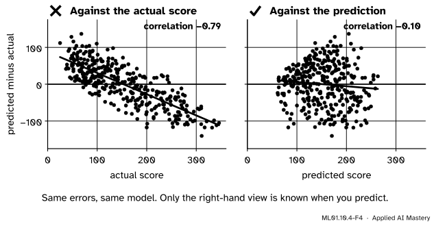
ML01.10.4-F4
Wrong beside right. Plotted against the outcome, even a sound model looks biased. Plotted against its own prediction, this one is level, though the cloud is wider on the right.
“The model predicts too low for the sickest patients, so it is biased against them.”
Sorted by outcome, even a sound model shows that slope: Result 3. Nobody knows the outcome when the prediction is made. Group by features and by the prediction itself. Those groups can be acted on.
“The test score disappointed me, so I tuned some more and tested again.”
The second test score is a validation score: it took part in a choice. Its honesty is gone, and nothing in the data can restore it. If the model must change after the test, say so in the report, or collect new test data.
“On the test set the error is 49.7 for sex code 1 and 39.5 for code 2. The model is unfair.”
Those groups hold 51 and 38 patients, with standard errors of \(5.4\) and \(4.1\). The gap is \({10.2 \pm 6.8}\). On the 353 working patients the two codes scored \(45.8\) and \(46.8\). Small groups are noisy. Give every group result with its size and its standard error.
Check yourself
Recall
1. What is an out-of-fold prediction, and why use it for error analysis?
Show answer
A prediction for a working row made by a model trained on the other folds. It shows the model’s errors on rows it has not seen, without opening the test set.
2. How is the overall MAE related to the MAEs of groups that cover every patient once?
Show answer
It is their weighted mean, each group weighted by its share of the patients.
3. For a least-squares model on its training rows, what is the correlation of the errors with the predictions, and with the targets?
Show answer
Zero with the predictions, and \(-\sqrt{1 - R^2}\) with the targets.
4. How many times is the test set used, and for what?
Show answer
Once, after every choice is final, to estimate how the chosen model will do on new data.
5. Name the five parts of the report.
Show answer
Question, data, method, result, limits.
Exercises
1.★ A model has an MAE of \(30\) on a group of 40 patients and \(50\) on a group of 60. What is its MAE on all 100? A colleague reports only that number. What is lost?
Show solution
\({(40 \times 30 + 60 \times 50)/100} = 4200/100 = 42\). The number \(42\) describes neither group: one is predicted much better and the other much worse.
2.★★ On a test set of 100 patients the absolute errors have mean \(20\) and standard deviation \(15\). (a) Give the standard error and a 95 percent interval, using \(t = 1.98\). (b) How many test patients would halve the width of the interval?
Show solution
(a) The standard error is \(15/\sqrt{100} = 1.5\). The interval is \({20 \pm 1.98 \times 1.5}\), that is \({20 \pm 2.97}\): from \(17.0\) to \(23.0\).
(b) The width is proportional to \(1/\sqrt{n}\). To halve it, \(\sqrt{n}\) must double, so \(n\) must be four times as large: 400 patients.
3.★★★ Use Result 3 to show that, for a least-squares model on its training rows, \(\text{Var}(y) = {\text{Var}(\hat{y}) + \text{Var}(e)}\), and so \(\text{sd}(\hat{y}) = \sqrt{R^2}\,\text{sd}(y)\). With \(\text{sd}(y) = 76\) and \(R^2 = 0.51\), how spread out are the predictions? Which feature of the anchor figure does this explain?
Show solution
Since \(y = {\hat{y} - e}\), expanding the variance of a difference as in lesson 3 gives \(\text{Var}(y) = {\text{Var}(\hat{y}) + \text{Var}(e)} - {2\,\text{Cov}(e, \hat{y})}\). Result 3 says the covariance is zero, which leaves \(\text{Var}(y) = {\text{Var}(\hat{y}) + \text{Var}(e)}\).
Divide by \(\text{Var}(y)\): \(1 = {\text{Var}(\hat{y})/\text{Var}(y)} + {(1 - R^2)}\), so \(\text{Var}(\hat{y}) = R^2\,\text{Var}(y)\) and \(\text{sd}(\hat{y}) = \sqrt{R^2}\,\text{sd}(y)\).
With the numbers: \({\sqrt{0.51} \times 76} = {0.714 \times 76} = 54\). The predictions are only about seven tenths as spread out as the truth. That is why the cloud in the anchor figure is narrower from left to right than it is tall: the predictions span about 200 points and the actual scores over 300.
Summary card
Find out for whom the model is wrong. Open the test set once. Report the number with its interval and its limits.
ML01.10.4-F1
Errors are distances from the line.
Groups.\(\text{MAE} = \sum_g \frac{n_g}{n}\,\text{MAE}_{G_g}\). Group by what is known when predicting.
Errors and targets. For least squares, \(r_{e,\hat{y}} = 0\) and \(r_{e,y} = -\sqrt{1 - R^2}\).
Test score.\({\bar{a} \pm t\,s/\sqrt{n}}\), measured once.
This project. Test MAE \(45.3\), interval \(38.3\) to \(52.4\), baseline \(66.3\). Error \(37\) for BMI under 25, \(52\) above.
Sources and next steps
Sources. Each was opened and checked against this lesson on 12 November 2026.
Margaret Mitchell and eight co-authors, Model Cards for Model Reporting, 2019. Section 4.7 asks for results “disaggregated”, broken down by chosen factors, with confidence intervals where possible. Section 4.4 asks how uncertainty was measured. Section 4.9 is “Caveats and Recommendations”.
Trevor Hastie, Robert Tibshirani and Jerome Friedman, The Elements of Statistical Learning, 2nd edition, Section 7.2 (page 222). If the test set is used repeatedly to choose the model, its error “will underestimate the true test error, sometimes substantially”.
NIST/SEMATECH e-Handbook of Statistical Methods. Section 1.3.5.2 gives the confidence limits for a mean, \({\bar{Y} \pm t\,s/\sqrt{N}}\), and their long-run meaning. Section 4.4.4.2 recommends plotting residuals against the predicted values to see whether their spread is constant.
scikit-learn 1.9 user guide, Section 3.1.1.2: cross_val_predict returns one prediction per row, each made when that row was held out, and is meant for inspecting predictions, not for the headline score.
SciPy documentation, scipy.stats.bootstrap: a two-sided bootstrap confidence interval, with the percentile method among its options.
Next. This is the last lesson of Machine Learning Foundations. Course ML02, Supervised Learning, adds stronger models: trees, ensembles and kernels. The four stages stay the same.