Look before you model: the range of every column, the gaps, the shape of the target and what moves with it. Then prepare the features inside a pipeline, so that every number it learns comes from training rows only and nothing leaks from the rows held out.
Summarise a table before modelling: the range of each column, its missing values, the shape of the target and the correlation of each feature with it.
Fill a missing value and standardise a feature by hand, using numbers learned from the training rows only.
Build a scikit-learn pipeline and explain why it prevents leakage during cross-validation.
Show with numbers how choosing features before the folds are cut makes pure noise look useful.
In review. The maths and code on this page are checked by automated tests on every change, but an independent reader has not signed it off yet. Spot a mistake or a confusing step? Tell us.
The question
You have 353 patients and eleven columns, and you have not looked at a single value yet. What should you check before fitting anything? And when the features need filling, scaling or choosing, how do you do it so that the patients held out for scoring cannot whisper to the model?
From the last lesson
1. Which constant prediction has the lowest mean absolute error?
Show answer
The median of the training targets. (The mean has the lowest squared error.)
2. What is this project’s baseline, and on which rows was it scored?
Show answer
An MAE of \({64.83 \pm 1.78}\), by five-fold cross-validation on the 353 working rows. The 89 test rows were set aside first and have not been opened.
Intuition
Preparing data means computing numbers from it: a median to fill gaps, a mean and a standard deviation to rescale, a list of the columns worth keeping. Each of those numbers is learned, just as a weight is. So the rule for weights applies to them as well: learn from the training rows, and only apply to the rows held out.
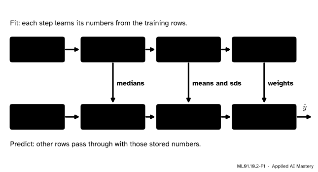
A pipeline enforces that rule. It chains the preparation steps and the model into one object with one fit and one predict.
ML01.10.2-F1
A pipeline. Fitting it (top row) learns every number from the training rows. Predicting with it (bottom row) only applies those numbers. The orange arrows point down, never up.
Before building one, look at the data. Looking tells you which steps the pipeline needs.
Build it up
Step 1. Split, then look. The test rows were locked away in lesson 1, before anything was drawn or summarised. That order matters: a histogram of all 442 targets would already show you the test rows, and every later choice would carry that knowledge. Everything in this lesson uses the 353 working rows.
Step 2. Read each column. For every column ask: what is it, in what units, over what range?
Column
What it is
Range
age
age in years
19 to 79
sex
a code, 1 or 2
184 and 169 patients
bmi
body mass index
18.0 to 42.2
bp
average blood pressure
62 to 133
s1, s2, s3
cholesterol: total, LDL, HDL
22 to 300
s4
total cholesterol / HDL
2.0 to 9.1
s5
log of triglycerides (probably)
3.3 to 6.1
s6
blood sugar
58 to 124
Three things stand out. Some columns span a few units and others a few hundred, so any method that measures distance needs them rescaled (ML01.3.3). sex is a code, not a quantity, and the documentation does not say which code is which. And s4 is not a new measurement: it is s1 divided by s3, mostly rounded to a whole number.
Step 3. Count the gaps. A missing value is usually stored as NaN. This table has none. Gaps can also hide as an impossible value such as \(0\) or \(-1\), so check the lowest and highest value of every column too. Here they are all plausible.
Step 4. Look at the target. Its histogram shows what the model has to predict.
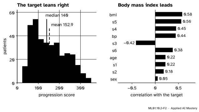
ML01.10.2-F2
What looking shows. Left: the target has a long right tail, so its mean is above its median. Right: each feature’s correlation with the target. No single feature comes close to \(1\).
The scores pile up between 50 and 100 and tail off slowly to the right. That is why the median, \(140\), is below the mean, \(152.9\).
Step 5. Look at what moves with the target. The correlation\(r\) of two columns is a number from \(-1\) to \(1\) that says how closely one follows a straight line in the other. Body mass index leads with \(0.58\), then s5 with \(0.56\). sex is last with \(0.05\). Among the features themselves, s1 and s2 have \(r = 0.88\): they nearly repeat each other.
Step 6. Prepare inside a pipeline. The table needs scaling. It needs no filling today, but next year’s table may have gaps, so the pipeline gets a filling step as well.
The formal statement
NoteDefinition: preparation step, and leakage
A preparation step has two parts. Fit computes numbers from the training rows. Transform applies those numbers to any rows. Leakage is the use, in building a model, of information that will not be available when it predicts. A step fitted on rows that are later used for scoring is a leak.
The two steps used here, for one feature with training values \(x_1, \dots, x_n\):
Fill replaces a missing value by \(m\), the median of the training values that are present.
Standardise replaces \(x\) by
\[
z = \frac{\cdata{x} - \cparam{\mu}}{\cparam{\sigma}},
\]
where \(\mu\) and \(\sigma\) are the mean and the standard deviation of the filled training values. The numbers \(m\), \(\mu\) and \(\sigma\) are learned once. A held-out value is transformed with the same three.
Result 1: a standardised training column has mean 0 and standard deviation 1. The mean of the \(z_i\) is
This holds for the rows that \(\mu\) and \(\sigma\) came from. Held-out rows come out near\(0\) and \(1\), not exactly, and that is correct: they are measured with someone else’s ruler.
Result 2: correlation is the average product of standardised values. For two columns with means \(\mu_x, \mu_y\) and standard deviations \(\sigma_x, \sigma_y\), the correlation is defined as the covariance divided by both standard deviations:
The second line only moves \(\sigma_x\) and \(\sigma_y\) inside the sum. So \(r\) is large and positive when patients above average in one column tend to be above average in the other. Changing the units of a column changes neither its standardised values nor \(r\).
Result 3: a pipeline is one function with one set of learned numbers. Write \(F\) for fill, \(S\) for standardise and \(f\) for the model. Fitting on training rows fixes the numbers inside each. The prediction for any row \(\vect{x}\) is then
In cross-validation the whole chain is fitted again in every round, on that round’s training folds. No number inside it has ever seen the fold being scored.
Go deeper: does every step leak equally?
No. A step that never looks at the target, such as scaling, leaks little: all it can learn from the held-out rows is where their features lie. The Elements of Statistical Learning even permits such “unsupervised” screening before the folds are cut. A step that uses the target, such as keeping the features most correlated with it, leaks badly: it is tuned to the very answers it will be scored on. The code below measures both leaks. A pipeline removes the need to tell them apart.
Worked example
Prepare one feature by hand. Five training patients have a body mass index of \(19\), \(23\), missing, \(27\) and \(31\). One held-out patient has \(35\). (The numbers are invented for this lesson, inside the real range.)
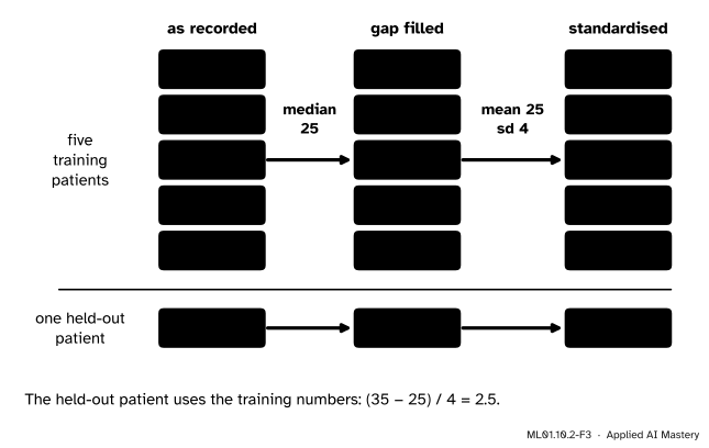
ML01.10.2-F3
Fill, then standardise. The three learned numbers, in orange, come from the training rows and are reused for the held-out patient.
Fit, on the training rows. The four values present are \(19, 23, 27, 31\). Their median is halfway between the middle two: \(m = {(23 + 27)/2} = 25\). Fill the gap: \(19, 23, 25, 27, 31\). The mean is \(125/5 = 25\). The deviations are \(-6, -2, 0, 2, 6\), with squares \(36, 4, 0, 4, 36\) and mean \(80/5 = 16\), so \(\sigma = 4\).
Transform the training rows. Subtract \(25\) and divide by \(4\): \(-1.5, -0.5, 0, 0.5, 1.5\). As Result 1 says, they average \(0\), and their squares \(2.25, 0.25, 0, 0.25, 2.25\) average \(5/5 = 1\).
Transform the held-out patient.\(z = {(35 - 25)/4} = 2.5\): two and a half training standard deviations above the training mean. A held-out patient with a missing value would be filled with \(25\) and get \(z = 0\).
The leak, for comparison. Fit on all six patients instead. The median of \(19, 23, 27, 31, 35\) is \(27\), the filled values \(19, 23, 27, 27, 31, 35\) have mean \(162/6 = 27\) and squared deviations \(64, 16, 0, 0, 16, 64\), mean \(160/6 = 26.67\), so \(\sigma = 5.16\). The held-out patient now gets \(z = {(35 - 27)/5.16} = 1.55\). By joining the fit, the patient has pulled the mean towards itself and stretched the ruler, and looks more ordinary than it is.
Code
First, look. pandas summarises every column of the working rows in a few lines.
import numpy as npimport pandas as pdfrom sklearn.datasets import load_diabetesfrom sklearn.model_selection import train_test_splitdata = load_diabetes(scaled=False, as_frame=True) # the table as a pandas DataFramework, test = train_test_split(data.frame, test_size=89, random_state=10) # the split of lesson 1print("working rows:", work.shape, " test rows, not opened:", len(test))summary = work.describe().T[["min", "50%", "max"]]summary["missing"] = work.isna().sum()print(summary.round(1).to_string())print("sex codes:", work["sex"].value_counts().to_dict())print("correlation of s4 with s1 / s3:", round(np.corrcoef(work["s4"], work["s1"] / work["s3"])[0, 1], 2)," share of s4 that is a whole number:", round(float((work["s4"] %1==0).mean()), 2))
working rows: (353, 11)   test rows, not opened: 89
         min    50%    max  missing
age     19.0   50.0   79.0        0
sex      1.0    1.0    2.0        0
bmi     18.0   25.8   42.2        0
bp      62.0   93.0  133.0        0
s1      97.0  187.0  300.0        0
s2      47.2  113.8  242.4        0
s3      22.0   47.0   99.0        0
s4       2.0    4.0    9.1        0
s5       3.3    4.6    6.1        0
s6      58.0   92.0  124.0        0
target  25.0  140.0  346.0        0
sex codes: {1.0: 184, 2.0: 169}
correlation of s4 with s1 / s3: 0.98   share of s4 that is a whole number: 0.85
Next, the relationships: Result 2 by hand for one feature, then corr for all of them.
def standardise(column):return (column - column.mean()) / column.std()bmi, target = work["bmi"].to_numpy(), work["target"].to_numpy()print("r of bmi with the target, as an average product:", round(np.mean(standardise(bmi) * standardise(target)), 2))r = work.corr()["target"].drop("target")print(r.sort_values(key=abs, ascending=False).round(2).to_string())between = work.drop(columns="target").corr()print("s1 with s2:", round(between.loc["s1", "s2"], 2), " s3 with s4:", round(between.loc["s3", "s4"], 2))
r of bmi with the target, as an average product: 0.58
bmi    0.58
s5     0.56
s4     0.45
bp     0.44
s3    -0.42
s6     0.38
age    0.22
s1     0.22
s2     0.18
sex    0.05
s1 with s2: 0.88   s3 with s4: -0.75
Now prepare. From scratch, a step is a pair of functions: one learns the numbers, one applies them.
def fit_prepare(column):"""Learn the three numbers of 'fill, then standardise' from a training column.""" median = np.nanmedian(column) # the median of the values that are present filled = np.where(np.isnan(column), median, column)return median, filled.mean(), filled.std()def apply_prepare(column, numbers): median, mean, sd = numbersreturn (np.where(np.isnan(column), median, column) - mean) / sdbmi_train = np.array([19.0, 23.0, np.nan, 27.0, 31.0])bmi_held = np.array([35.0, np.nan]) # one patient with a value, one withoutnumbers = fit_prepare(bmi_train)print("learned from the training rows (median, mean, sd):", [float(v) for v in numbers])print("training rows:", apply_prepare(bmi_train, numbers))print("held-out rows:", apply_prepare(bmi_held, numbers))leaky = fit_prepare(np.append(bmi_train, 35.0)) # wrong: the held-out patient joins the fitprint("leaky numbers:", np.round(leaky, 2), " held-out patient:", np.round(apply_prepare(bmi_held, leaky), 2))
learned from the training rows (median, mean, sd): [25.0, 25.0, 4.0]
training rows: [-1.5 -0.5  0.   0.5  1.5]
held-out rows: [2.5 0. ]
leaky numbers: [27.   27.    5.16]   held-out patient: [1.55 0.  ]
The library versions are SimpleImputer and StandardScaler, and make_pipeline chains them to a model. Here the model is \(k\)-nearest neighbours with \(k = 5\), the method of ML01.3.4 that needs scaling most.
from sklearn.impute import SimpleImputerfrom sklearn.model_selection import KFold, cross_val_scorefrom sklearn.neighbors import KNeighborsRegressorfrom sklearn.pipeline import make_pipelinefrom sklearn.preprocessing import StandardScalerprepare = make_pipeline(SimpleImputer(strategy="median"), StandardScaler()).fit(bmi_train.reshape(-1, 1))print("stored by the library:", prepare[0].statistics_, prepare[1].mean_, prepare[1].scale_," held-out:", prepare.transform(bmi_held.reshape(-1, 1)).ravel())X_work, y_work = work.drop(columns="target").to_numpy(), work["target"].to_numpy()cv = KFold(n_splits=5) # the five folds of lesson 1def cv_mae(model, X):return-cross_val_score(model, X, y_work, cv=cv, scoring="neg_mean_absolute_error").mean()pipeline = make_pipeline(SimpleImputer(strategy="median"), StandardScaler(), KNeighborsRegressor(n_neighbors=5))print(f"k-NN on raw features: {cv_mae(KNeighborsRegressor(n_neighbors=5), X_work):.2f}")print(f"k-NN in a pipeline: {cv_mae(pipeline, X_work):.2f}")scaled_first = StandardScaler().fit_transform(X_work) # wrong: scaled with all 353 rows, then cut into foldsprint(f"k-NN, scaled before the folds: {cv_mae(KNeighborsRegressor(n_neighbors=5), scaled_first):.2f}")
stored by the library: [25.] [25.] [4.]  held-out: [2.5 0. ]
k-NN on raw features:           53.63
k-NN in a pipeline:             47.41
k-NN, scaled before the folds:  47.39
The library stores the same three numbers. On the real table, scaling takes \(k\)-NN from an MAE of \(53.63\) to \(47.41\): well below the baseline’s \(64.83\). Scaling before the folds are cut gives \(47.39\). That leak is worth \(0.02\), because scaling never looks at the target.
A step that does look at the target leaks far more. Make 2,000 columns of random numbers, keep the ten that correlate best with the target, and cross-validate a linear model on them.
from sklearn.feature_selection import SelectKBest, f_regressionfrom sklearn.linear_model import LinearRegressionnoise = np.random.default_rng(10).normal(size=(353, 2000)) # 2,000 columns of pure noisedef correlations(table, target): centred = table - table.mean(axis=0)return centred.T @ (target - target.mean()) / (len(target) * table.std(axis=0) * target.std())r_noise = correlations(noise, y_work)chosen = np.argsort(np.abs(r_noise))[-10:] # wrong: chosen with all 353 rowsprint(f"standard deviation of r for noise: {r_noise.std():.3f} the ten largest: {np.abs(r_noise[chosen]).min():.2f} to {np.abs(r_noise).max():.2f}")print(f"chosen on all rows, then cross-validated: {cv_mae(LinearRegression(), noise[:, chosen]):.2f}")inside = make_pipeline(SelectKBest(f_regression, k=10), LinearRegression())print(f"chosen inside each fold, by a pipeline: {cv_mae(inside, noise):.2f}")
standard deviation of r for noise: 0.055   the ten largest: 0.15 to 0.21
chosen on all rows, then cross-validated:  55.61
chosen inside each fold, by a pipeline:    70.44
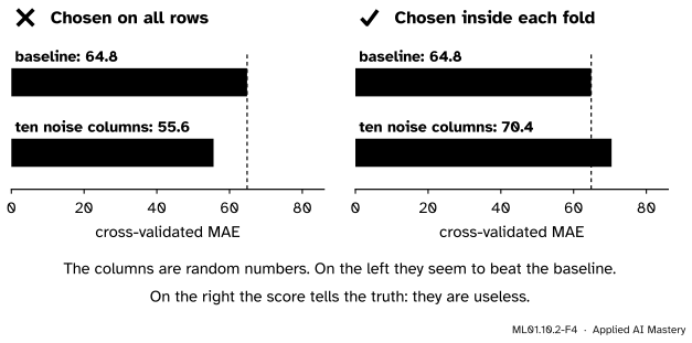
The noise columns’ correlations with the target have a standard deviation of \(0.055\). But the best ten of 2,000 reach \(0.15\) to \(0.21\), by luck alone. Chosen on all the rows, they score \(55.61\) and seem to beat the baseline. Chosen inside each fold, they score \(70.44\), worse than the baseline: the truth about random numbers.
Explore
This module’s interactive, the project board, is in lesson 3. Its second stage is this lesson’s choice: switch between Raw features and Standardised and watch what scaling does to \(k\)-nearest neighbours, to a penalised linear model, and to plain linear regression (nothing).
Pitfalls
ML01.10.2-F4
Wrong beside right. The same ten-out-of-2,000 selection, done before the folds are cut (left) and inside each fold (right).
“I cross-validated, so my score is honest.”
Only if everything that learned from data was inside the cross-validation. Any step done once on all the rows, before the folds were cut, has seen every fold. Put the steps in a pipeline and cross-validate the pipeline.
“There is no NaN, so nothing is missing.”
A gap can be stored as \(0\), \(-1\) or \(999\). A blood pressure of \(0\) is not a measurement. Check the lowest and highest value of every column against what is physically possible.
“sex has a correlation of 0.05, so it is useless.”
A correlation looks at one feature at a time, and only for a straight-line link. A feature can matter once the others are accounted for: the model chosen in lesson 3 keeps sex. And a code is not a quantity. With two codes a linear model copes, but a column coded 1, 2, 3 for three groups would need one yes-or-no column for each.
Check yourself
Recall
1. Name four things to check in a table before fitting any model.
Show answer
What each column is and its range, whether values are missing, the shape of the target, and how each feature relates to the target (and to the other features).
2. From which rows are the median, the mean and the standard deviation of a preparation step computed?
Show answer
From the training rows only. Held-out rows are transformed with those same numbers.
3. What does a pipeline’s fit do, and what does its predict do?
Show answer
fit learns the numbers of every step, in order, from the rows it is given. predict passes new rows through the steps with the stored numbers and returns the model’s predictions.
4. Why did scaling before the folds leak only 0.02, while choosing features before the folds leaked 15?
Show answer
Scaling never uses the target, so it learns almost nothing useful from the held-out rows. Choosing features by their correlation with the target is tuned to the held-out answers themselves.
5. What is the correlation \(r\) in terms of standardised values?
Show answer
The average, over the examples, of the product of the two standardised values.
Exercises
1.★ Four training patients have blood pressures \(80\), \(90\), \(110\) and \(120\). Find the training mean and standard deviation, standardise the four values, and standardise a held-out patient with \(130\).
Show solution
The mean is \(400/4 = 100\). The deviations are \(-20, -10, 10, 20\), with squares \(400, 100, 100, 400\) and mean \(1000/4 = 250\), so \(\sigma = \sqrt{250} = 15.81\). The standardised values are \(-1.26, -0.63, 0.63, 1.26\). The held-out patient gets \({(130 - 100)/15.81} = 1.90\).
2.★★ A training column has the values \(4\), missing, \(10\), \(6\), missing, \(40\). (a) Fill it with the median, and then with the mean, of the values present. (b) Which filling is affected more by the value \(40\)? (c) What should a missing value in a test row be filled with?
Show solution
(a) The values present are \(4, 6, 10, 40\). Their median is \({(6 + 10)/2} = 8\) and their mean is \(60/4 = 15\). Filled with the median: \(4, 8, 10, 6, 8, 40\). With the mean: \(4, 15, 10, 6, 15, 40\).
(b) The mean. Without the \(40\) the values \(4, 6, 10\) have mean \(6.67\) and median \(6\): the outlier moved the mean by \(8.33\) and the median by \(2\). That is why the median is the safer default.
(c) With the training median, \(8\). The test row’s own column plays no part.
3.★★★ Show that standardising two columns does not change their correlation, and that the least-squares line through the standardised points has slope \(r\). Use the slope formula of ML01.4.2, covariance over variance.
Show solution
Let \(u_i = {(x_i - \mu_x)/\sigma_x}\) and \(v_i = {(y_i - \mu_y)/\sigma_y}\). By Result 1 each has mean \(0\) and standard deviation \(1\). Their correlation is their covariance divided by both standard deviations:
The least-squares slope of \(v\) on \(u\) is the covariance of \(u\) and \(v\) divided by the variance of \(u\). The covariance is \(\frac{1}{n}\sum_i u_i v_i = r\) and the variance of \(u\) is \(1\), so the slope is \(r/1 = r\). For body mass index, one standard deviation more goes with \(0.58\) standard deviations more of the progression score.
Summary card
Every number a preparation step uses is learned, so it is learned from training rows only.
ML01.10.2-F1
Learn above, apply below.
Look first. Ranges, gaps, the shape of the target, correlations. On the working rows only.
Standardise.\(z = {(x - \mu)/\sigma}\), with \(\mu\) and \(\sigma\) from the training rows.
Correlation.\(r\) is the average product of standardised values.
Pipeline.\(\hat{y} = f(S(F(\vect{x})))\), refitted in every round of cross-validation.
This project.\(k\)-NN: \(53.63\) raw, \(47.41\) in a pipeline. Noise chosen before the folds: \(55.61\). Inside: \(70.44\).
Sources and next steps
Sources. Each was opened and checked against this lesson on 12 November 2026.
scikit-learn 1.9 user guide. Section 12.2, Data leakage, defines leakage as using information that would not be available at prediction time, gives the rule never to call fit on the test data, and shows feature selection on random data scoring 0.76 before the split and 0.5 after it. Section 8.1.1 lists safety among the purposes of a Pipeline. Section 3.1.1 says preprocessing should be learnt from a training set and applied to held-out data. Section 9.1.2 gives each column’s meaning, with s5 as “possibly log of serum triglycerides level”.
Trevor Hastie, Robert Tibshirani and Jerome Friedman, The Elements of Statistical Learning, 2nd edition, Section 7.10.2, “The Wrong and Right Way to Do Cross-validation”. With 50 samples and 5,000 noise predictors, screening before cross-validation gives an error of 3 percent where the truth is 50 percent. Unsupervised screening may be done before samples are left out.
scikit-learn 1.9 documentation, StandardScaler (\(z = {(x - u)/s}\) from the training samples) and SimpleImputer (the median strategy).
Bradley Efron, Trevor Hastie, Iain Johnstone and Robert Tibshirani, Least Angle Regression, Table 1: the first rows of the table, with sex coded 1 and 2 and no key.