Every threshold gives a different confusion matrix. Build the ROC curve and the precision-recall curve point by point from ten scores, read the area under the ROC curve as the chance that a positive outranks a negative, and learn when the second curve tells you more.
Compute the true positive rate and the false positive rate at a threshold, and plot the point they give.
Build a ROC curve and a precision-recall curve step by step from a table of scores.
Show that the area under the ROC curve is the share of positive-negative pairs that the model puts in the right order.
Explain why a ROC curve does not change when one class becomes rarer, and why precision does.
Decide when to read the precision-recall curve in place of the ROC curve.
In review. The maths and code on this page are checked by automated tests on every change, but an independent reader has not signed it off yet. Spot a mistake or a confusing step? Tell us.
The question
A model gives every student a probability of passing. Each threshold turns those into answers, with its own precision and recall. Suppose nobody has chosen the threshold yet, or two teams will choose differently. Can you judge the model itself, at every threshold at once, in one picture and one number?
From the last lesson
1. Write precision and recall in terms of the counts.
2. You lower the threshold. What happens to recall, and what usually happens to precision?
Show answer
Recall rises or stays the same. Precision usually falls.
Intuition
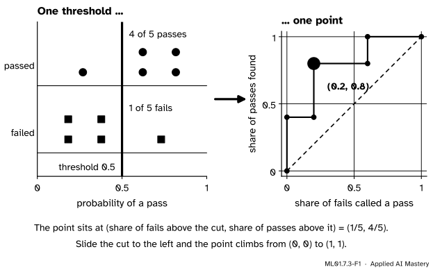
A classifier such as logistic regression first gives each example a score, here a probability, that is higher when the model leans towards “positive”. The threshold is a cut through the scores.
For any cut, ask two things. What share of the positives lies above it? That is the recall of the last lesson, also called the true positive rate. What share of the negatives lies above it? That is the false positive rate. Plot the second across and the first up, and the cut becomes a point.
ML01.7.3-F1
The ten students of module ML01.6. Four of the five passes and one of the five fails are above the cut at \(0.5\): the point \({(0.2,\ 0.8)}\).
Slide the cut through every position and the point traces a path: the ROC curve. The name, receiver operating characteristic, comes from signal detection theory, which used this picture long before machine learning did.
Build it up
Step 1. Two rates. With \(P\) actual positives and \(N\) actual negatives, the true positive rate is \(\text{TP} / P\) and the false positive rate is \(\text{FP} / N\). At threshold \(0.5\) the students give \({4/5 = 0.8}\) and \({1/5 = 0.2}\).
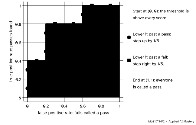
Step 2. Sort by score, highest first. Two passes at \(0.818\), a fail at \(0.731\), two passes at \(0.622\), two fails at \(0.378\), a pass at \(0.269\) and two fails at \(0.182\).
Step 3. Start above every score. Nothing is flagged, so both rates are \(0\): the point \({(0, 0)}\).
Step 4. Lower the threshold past one student at a time. A student who passed is one more positive found: the point steps up by \(1/P\). A student who failed is one more negative flagged: it steps right by \(1/N\). Students with the same score move together.
ML01.7.3-F2
The ROC curve of the ten students, one student to a step, in order of score.
Step 5. End below every score. Everyone is flagged and both rates are \(1\). Every ROC curve runs from \({(0, 0)}\) to \({(1, 1)}\).
Step 6. Read the curve. A perfect model ranks every positive above every negative: its curve goes straight up to \({(0, 1)}\) and then across. Scores that carry no information flag both classes at about the same rate, so their curve stays close to the diagonal. The area under the curve, the AUC, is \(1\) for a perfect ranking and about \(0.5\) for no information. For the students it is \(0.80\).
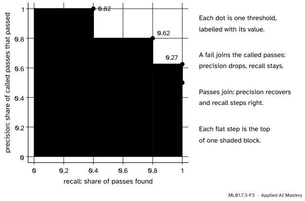
Step 7. The other curve. In the same sweep, plot precision against recall at each threshold. That is the precision-recall curve.
ML01.7.3-F3
The precision-recall curve of the same students, drawn as steps. It ends where everyone is called a pass and the precision is the share of passes, \(0.5\).
Step 8. Which curve? Each rate of the ROC curve is computed inside one class, so the curve ignores how many negatives there are for each positive. Precision does: it sets true positives beside false positives. When rare positives are what you are after, the precision-recall curve shows a weakness that the ROC curve hides.
The formal statement
NoteDefinition: ROC curve and AUC
A model gives example \(i\) a score \(s_i\). For a threshold \(c\) on the score, call an example positive when \({s_i \ge c}\), and count TP and FP. With \(P\) actual positives and \(N\) actual negatives,
The ROC curve joins the points \({\big(\text{FPR}(c),\ \text{TPR}(c)\big)}\) as \(c\) falls from above every score to below every score. The AUC is the area under it.
Result 1: the AUC counts pairs. Assume first that no positive has the same score as a negative. Going down the sorted list, the curve moves right only when the threshold passes a negative, by a step of width \(1/N\). During the step for negative \(j\) the height of the curve is the number of positives already passed, divided by \(P\). Those positives are exactly the ones that score higher than negative \(j\). Call their number \(h_j\). The step adds a rectangle of area \({\frac{1}{N} \times \frac{h_j}{P}}\), and all the steps together add
The top counts every pair of one positive and one negative in which the positive scores higher. The bottom is the number of all such pairs. So the AUC is the share of the pairs that the model puts in the right order: the probability that a randomly chosen positive outscores a randomly chosen negative.
Result 2: the ROC curve ignores the class balance, and precision does not. Let \({\rho = P / n}\) be the share of positives among the \({n = P + N}\) examples. By definition \({\text{TP} = \text{TPR} \cdot P}\) and \({\text{FP} = \text{FPR} \cdot N}\). Put these into the precision, then divide top and bottom by \(n\):
Copy every negative twenty times. Each copy is above or below the threshold as before, so TPR, FPR and the ROC curve do not change. But \(\rho\) falls, the term \({(1 - \rho)\,\text{FPR}}\) grows against \({\rho\,\text{TPR}}\), and precision drops at every threshold that flags both true and false positives.
Result 3: scores with no information. If the scores have nothing to do with the classes, a threshold flags the same share \(t\) of both classes, on average. Then \({\text{TPR} = \text{FPR} = t}\): the diagonal, with area \(0.5\). In Result 2 this gives
So on a precision-recall plot the no-information line is horizontal, at the share of positives: \(0.5\) for the students, \(0.01\) for the payments of lesson 1.
Average precision. The precision-recall curve has its own summary. List the thresholds from the highest down, with recall \(\text{rec}_k\) and precision \(\text{prec}_k\) at the \(k\)-th one, and \({\text{rec}_0 = 0}\). The average precision is
Each rise in recall is weighted by the precision at which it was won. It is exactly the area under the curve drawn as steps, as in Step 7. Only the dots come from thresholds.
Go deeper: ties, and why only the order of the scores matters
Ties. A positive and a negative with the same score pass the threshold together, and the curve moves along a slanted segment. Half of that step’s rectangle lies under it, so a tied pair counts as half a pair in Result 1.
Order. Result 1 only ever compares scores. Apply any function that keeps them in the same order, such as squaring the probabilities, and the ROC curve and the AUC do not change. So the AUC measures how well the model ranks. It does not say whether a score of \(0.8\) means “passes four times in five”, or which threshold to use.
Worked example
The sweep, by hand. There are \({P = 5}\) passes and \({N = 5}\) fails.
Cut
Who joins
TP, FP
(FPR, TPR)
above \(0.818\)
nobody
\(0,\ 0\)
\((0,\ 0)\)
\(0.818\)
2 passes
\(2,\ 0\)
\((0,\ 0.4)\)
\(0.731\)
1 fail
\(2,\ 1\)
\((0.2,\ 0.4)\)
\(0.622\)
2 passes
\(4,\ 1\)
\((0.2,\ 0.8)\)
\(0.378\)
2 fails
\(4,\ 3\)
\((0.6,\ 0.8)\)
\(0.269\)
1 pass
\(5,\ 3\)
\((0.6,\ 1)\)
\(0.182\)
2 fails
\(5,\ 5\)
\((1,\ 1)\)
The AUC as an area. Under the staircase are three rectangles, one for each horizontal run:
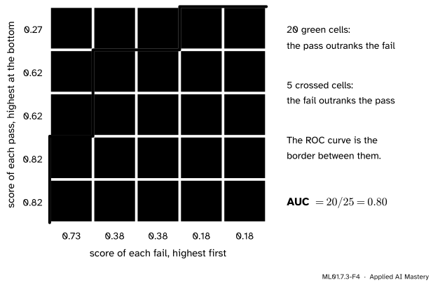
The AUC as pairs. There are \({5 \times 5 = 25}\) pairs of one pass and one fail. Each pass at \(0.818\) outranks all five fails: \(10\) pairs. Each pass at \(0.622\) outranks every fail except the one at \(0.731\): \(8\) pairs. The pass at \(0.269\) outranks only the two fails at \(0.182\): \(2\) pairs. That is \({10 + 8 + 2 = 20}\) pairs in the right order, and \({20 / 25 = 0.80}\).
ML01.7.3-F4
The square of the ROC plot, cut into one cell for each pair. A cell is under the curve exactly when its pass outranks its fail.
The precision-recall points. From the same counts:
Threshold
Recall
Precision
\(0.818\)
\(0.4\)
\(2/2 = 1\)
\(0.731\)
\(0.4\)
\(2/3 = 0.667\)
\(0.622\)
\(0.8\)
\(4/5 = 0.8\)
\(0.378\)
\(0.8\)
\(4/7 = 0.571\)
\(0.269\)
\(1\)
\(5/8 = 0.625\)
\(0.182\)
\(1\)
\(5/10 = 0.5\)
Recall rises three times, by \(0.4\), \(0.4\) and \(0.2\), at precisions \(1\), \(0.8\) and \(0.625\). So
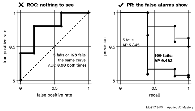
Now make the passes rare. Keep the five passes, and replace each fail by twenty fails with the same score: 100 fails. At threshold \(0.5\) the counts become \({\text{TP} = 4}\) and \({\text{FP} = 20}\). The rates are \({4/5 = 0.8}\) and \({20/100 = 0.2}\), the same point as before, and the ROC curve and its AUC of \(0.80\) are unchanged. The precision falls from \(0.8\) to \({4/24 = 0.167}\). Result 2 agrees: with \({\rho = 5/105}\),
Last, the detector of eights from lessons 1 and 2, with 44 eights among its 450 test images.
from sklearn.datasets import load_digitsfrom sklearn.linear_model import LogisticRegressionfrom sklearn.model_selection import train_test_splitfrom sklearn.pipeline import make_pipelinefrom sklearn.preprocessing import StandardScalerdigits = load_digits()is_eight = (digits.target ==8).astype(int)X_train, X_test, y_train, y_test = train_test_split( digits.data, is_eight, test_size=0.25, random_state=0, stratify=is_eight)model = make_pipeline(StandardScaler(), LogisticRegression(max_iter=1000)).fit(X_train, y_train)proba = model.predict_proba(X_test)[:, 1]print(f"share of eights in the test set: {y_test.mean():.3f}")print(f"AUC: {roc_auc_score(y_test, proba):.3f} by pairs: {auc_by_pairs(y_test, proba):.3f}")print(f"average precision: {average_precision_score(y_test, proba):.3f}")
share of eights in the test set: 0.098
AUC: 0.975   by pairs: 0.975
average precision: 0.892
An AUC of \(0.975\) says that in \(97.5\%\) of the pairs of an 8 and another digit, the 8 scores higher. That sounds nearly perfect. The average precision, \(0.892\), is soberer, and fits what lesson 2 found: at threshold \(0.5\) this model misses 12 of the 44 eights.
Explore
ML01.7-X1
Threshold slider
The histograms show the scores a model gives to 100 positive and 100 negative examples. Drag the threshold, or use the slider, and watch the four counts and the marked point on both curves. Then press Rare and Very rare: the ROC curve stays put and the precision-recall curve sinks. Last, pull the separation down to zero.
Pitfalls
ML01.7.3-F5
Wrong beside right. With twenty times as many fails the ROC curve is the same line. The precision-recall curve shows what happened: most of the model’s “passes” are now false alarms.
“The ROC curve looks excellent, so the alarms can be trusted.”
The ROC curve counts false positives as a share of all the negatives. When negatives outnumber positives a hundred to one, a tiny share of them can bury the true positives. Fraud, faults and diseases are all rare, so in machine learning this is common. If you will act on the alarms, read the precision-recall curve too.
“An AUC of 0.80 means the model is right 80% of the time.”
The AUC is not an accuracy, and involves no threshold. It says that in \(80\%\) of the pairs of one positive and one negative, the positive has the higher score.
“A high AUC means the default threshold of 0.5 is fine.”
The AUC depends only on the order of the scores. Square every probability and the ROC curve and the AUC are unchanged, yet a different set of examples now lies above \(0.5\). Choosing the threshold is a separate job, done with precision, recall and the costs of lesson 2.
Check yourself
Recall
1. Which two rates does a ROC curve plot, and on which axes?
Show answer
The false positive rate \(\text{FP}/N\) across and the true positive rate \(\text{TP}/P\) up, one point for each threshold.
2. Going down the list of scores, how does the curve move for a positive and for a negative?
Show answer
Up by \(1/P\) for a positive and right by \(1/N\) for a negative.
3. What does the AUC measure, as a probability?
Show answer
The probability that a randomly chosen positive has a higher score than a randomly chosen negative.
4. Where is the no-information line on a ROC plot, and where on a precision-recall plot?
Show answer
The diagonal, with area \(0.5\), on a ROC plot. The horizontal line at the share of positives on a precision-recall plot.
5. Negatives become twenty times as common. What happens to the ROC curve and to precision?
Show answer
The ROC curve does not move: each of its rates is computed inside one class. Precision falls.
Exercises
1.★ Six examples have these scores and true classes: \(0.9\) (positive), \(0.8\) (negative), \(0.7\) (positive), \(0.4\) (positive), \(0.3\) (negative), \(0.1\) (negative). List the points of the ROC curve and find the AUC in two ways.
Show solution
\({P = 3}\) and \({N = 3}\), so every step is \(\tfrac13\): up for a positive, right for a negative. In order of score that is up, right, up, up, right, right. The points are \({(0, 0)}\), \({(0, \tfrac13)}\), \({(\tfrac13, \tfrac13)}\), \({(\tfrac13, \tfrac23)}\), \({(\tfrac13, 1)}\), \({(\tfrac23, 1)}\) and \({(1, 1)}\).
Area. The three steps to the right are at heights \(\tfrac13\), \(1\) and \(1\): \(\tfrac13 \times \tfrac13 + \tfrac13 + \tfrac13 = \tfrac79 = 0.778\).
Pairs. The positive at \(0.9\) outranks all three negatives. Those at \(0.7\) and \(0.4\) outrank two each. That is \({3 + 2 + 2 = 7}\) of \(9\) pairs: \(0.778\).
2.★★ At its chosen threshold a fraud detector has a true positive rate of \(0.8\) and a false positive rate of \(32/990\). Use Result 2 to find its precision when the share of fraud is \(0.1\), \(0.01\) and \(0.001\).
The same point of the same ROC curve means \(73\%\), \(20\%\) or \(2.4\%\) of alarms right.
3.★★★ Assume no two scores are equal. Show that replacing each score \(s_i\) by \({-s_i}\) turns an AUC of \(A\) into \({1 - A}\). What does that say about a model with an AUC of \(0.2\)?
Show solution
By Result 1 the AUC is the share of positive-negative pairs in which the positive scores higher. Take a pair with scores \({s_+}\) and \({s_-}\). If \({s_+ > s_-}\) then \({-s_+ < -s_-}\), and the other way round. So every right pair becomes wrong and every wrong pair right, and the share of right pairs changes from \(A\) to \({1 - A}\).
A model with an AUC of \(0.2\) is not ignorant. It ranks four pairs in five the wrong way round, which takes information: reverse its scores and the AUC is \(0.8\).
Summary card
Sweep the threshold: each cut is a point, the points make a curve.
ML01.7.3-F1
One threshold, one point.
ROC curve.\(\text{FP}/N\) across, \(\text{TP}/P\) up. A positive is a step up, a negative a step right.
AUC. The share of positive-negative pairs in the right order. No information: \(0.5\). Ten students: \({20/25 = 0.80}\).
Precision-recall curve. Same sweep, precision against recall. No information: the share of positives.
Class balance.\(\text{precision} = \frac{\rho\,\text{TPR}}{\rho\,\text{TPR} + (1 - \rho)\,\text{FPR}}\). Only precision sees \(\rho\).
Rare positives. Twenty times the fails: AUC still \(0.80\), average precision down from \(0.845\) to \(0.482\).
Sources and next steps
Sources. Each was opened and checked against this lesson on 12 November 2026.
Tom Fawcett, An introduction to ROC analysis, Pattern Recognition Letters 27 (2006), pages 861 to 874. Section 1 traces ROC graphs to signal detection theory. Section 3.1 gives the diagonal of random guessing, and Section 5 builds the curve by going down the sorted scores. Section 4.2 states that ROC curves do not change with the proportion of positives to negatives, and Figure 5 shows precision-recall curves that do. Section 7 states that the AUC is the probability that a random positive is ranked above a random negative. Read in the copy hosted by the University of Houston.
scikit-learn 1.9 User Guide, Metrics and scoring: Section 3.4.4.15 (the ROC curve) and Section 3.4.4.9, which defines the average precision as \({\sum_n (R_n - R_{n-1}) P_n}\). The page for roc_curve counts a score at or above the threshold as positive and sets the first threshold to infinity. PrecisionRecallDisplay draws the curve as steps, to match the average precision.