Fit polynomials of rising degree to twelve noisy points. A straight line misses the pattern, a degree-11 curve passes through every point and learns the noise, and only held-back examples can say where between them to stop.
Fit a polynomial of any degree by least squares, as a linear model on the powers of the input.
Explain why the training error cannot rise when the degree rises, and why it reaches zero at degree n minus 1.
Recognise underfitting and overfitting in a picture of the fit and in a table of training and test errors.
Choose a degree with held-back examples, and say why the training error cannot make that choice.
In review. The maths and code on this page are checked by automated tests on every change, but an independent reader has not signed it off yet. Spot a mistake or a confusing step? Tell us.
The question
You have twelve noisy measurements. A straight line through them misses an obvious wave. A polynomial of degree 11 passes through all twelve exactly. Which would you trust with a thirteenth measurement? And how do you find the right model between the two when nobody tells you the answer?
Intuition
Module ML01.2 made a model more flexible by giving a table more bins, and watched the training error and the test error part company. This module explains why. It needs a family of models with a dial for flexibility, and the classic one is the polynomial.
Degree 0 is a flat line and degree 1 is the straight line of module ML01.4. Each extra degree adds one weight and lets the curve bend once more. Other families of models have such dials too: the number of bins of a table, the \(k\) of k-nearest neighbours, the size of a neural network. What the polynomial shows here happens, in some form, to all of them.
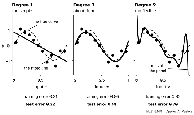
The data come from a source made up for this module. The input \(x\) lies between 0 and 1. The target is a wave, \(\sin(2\pi x)\), plus noise: a random number with mean 0 and standard deviation \(0.3\). Twelve examples from this source are the training set.
ML01.8.1-F1
The same twelve points, three polynomials. The fitted curve gets closer to the training points with every degree. It gets closer to the dashed true curve only up to a point.
The line is too stiff to follow the wave. That is underfitting. The degree-9 curve is so flexible that it follows the points themselves, noise included, and swings between and beyond them. That is overfitting. Degree 3 sits between: flexible enough for the wave, too stiff for the noise.
Build it up
Step 1. The twelve points. The inputs are the middles of twelve equal slices of the interval from 0 to 1. The targets, rounded to two decimals, are these.
\(x\)
\(y\)
\(x\)
\(y\)
\(0.042\)
\(0.18\)
\(0.542\)
\(-0.40\)
\(0.125\)
\(1.06\)
\(0.625\)
\(-1.11\)
\(0.208\)
\(0.84\)
\(0.708\)
\(-0.66\)
\(0.292\)
\(0.67\)
\(0.792\)
\(-1.37\)
\(0.375\)
\(0.33\)
\(0.875\)
\(-0.38\)
\(0.458\)
\(-0.02\)
\(0.958\)
\(-0.40\)
Step 2. A polynomial is a linear model in disguise. Treat \(x, x^2, \dots, x^d\) as \(d\) separate features. The prediction is then a weighted sum of features plus a bias, which is the model of lesson ML01.4.3. Its design matrix has a column of ones and one column for each power, and the best weights are the least-squares solution found there. The curve bends, but the model is still linear in its weights.
Step 3. Training error against degree. Fit every degree from 0 to 11 and score each fit on the twelve points. The training error falls at every step: \(0.525\), \(0.214\), \(0.202\), \(0.057\), and on down to \(0.019\) at degree 9 and exactly \(0\) at degree 11. Twelve weights can meet twelve demands.
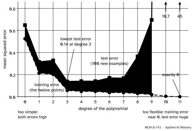
Step 4. Test error against degree. Draw 100 new examples from the same source and score the same fits on them.
ML01.8.1-F2
Training error only falls. Test error falls to \(0.14\) at degree 3, stays low up to degree 7, and then climbs out of the picture: \(10.7\) at degree 10 and \(45\) at degree 11.
The lowest test error is \(0.138\), at degree 3. No model can be expected to beat the noise: the true curve itself scores \(0.104\) on these 100 examples.
Step 5. Read the two regimes off the two errors. On the left, both errors are high: the model cannot even fit the points it was given. On the right, the training error is tiny and the test error is huge: the gap of lesson ML01.2.3 has swallowed everything. Good models live in the valley between.
A model underfits when it cannot reach a low error even on its training set. It overfits when its training error is low and its test error is much higher.
The textbook word for what the degree controls is capacity: the variety of functions a family can fit. Two results explain the training curve.
Result 1: the training error cannot rise when the degree rises. Let \(w_0, \dots, w_d\) be the best weights of degree \(d\). The polynomial of degree \({d + 1}\) with those weights and \(w_{d+1} = 0\) is the same function, so it has the same training error. The best polynomial of degree \({d + 1}\) is at least as good as that one. This is Result 1 of lesson ML01.1.3: a family never fits worse than a family inside it.
Result 2: with \(n\) different inputs, degree \({n - 1}\) has training error zero. Take examples \((x_1, y_1), \dots, (x_n, y_n)\) whose inputs are all different. For each \(i\), multiply together one factor for every other input:
At \(x_k\) every term vanishes except the \(k\)th, which is \({y_k \cdot 1}\). So \(p(x_k) = y_k\) for every \(k\): the polynomial \(p\), of degree at most \({n - 1}\), passes through all \(n\) points. Least squares at degree \({n - 1}\) does at least as well, so its training error is \(0\), and by Result 1 it stays \(0\) for every higher degree.
Nothing about the targets was used. They could be random numbers. Like the lookup table of lesson ML01.2.1, a polynomial of high enough degree fits perfectly any training set whose inputs are all different, so its perfect score tells you nothing.
No such rule holds for the test error. It usually traces a U, as in the figure, but only measurement on held-back examples shows where the bottom is.
Go deeper: why the flexible curve swings: every prediction is a weighted sum of the targets
The formula for \(p\) shows that a prediction is a weighted sum of the training targets, with weights \(\ell_i(x)\) that depend only on the inputs. The same is true of every least-squares fit, because the weights solve the normal equations of lesson ML01.4.3, whose right-hand side holds weighted sums of the targets.
For the twelve inputs of this lesson, take the prediction at \(x = 0\). The largest of its twelve weights is \(0.31\) for the line, \(1.02\) for the cubic, \(12.1\) for degree 9 and \(162\) for degree 11. Shift one target by \(0.1\), an ordinary bit of noise, and the degree-11 prediction at \(x = 0\) can move by \(16\). A stiff model averages the noise away. A flexible one amplifies it.
Worked example
Fit degrees 0, 1 and 3 to the course’s four points by hand, and test each fit.
The training points are \((1, 2)\), \((2, 3)\), \((3, 5)\), \((4, 6)\). The test set is the four new examples of lesson ML01.2.1: \((1.5, 3)\), \((2.5, 4)\), \((3.5, 5)\), \((4.5, 7)\).
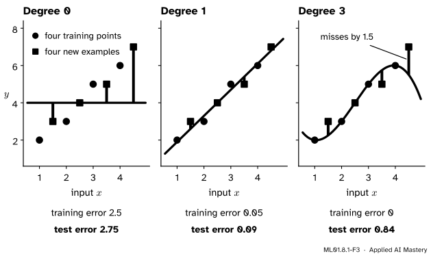
Degree 0. The best constant is the mean of the targets, \({(2 + 3 + 5 + 6)/4} = 4\). Its training error is \({(4 + 1 + 1 + 4)/4} = 2.5\). On the new examples the misses are \(1, 0, 1\) and \(3\), so the test error is \({(1 + 0 + 1 + 9)/4} = 2.75\).
Degree 1. The best line is \(\hat{y} = {1.4x + 0.5}\) (lesson ML01.4.2), with training error \(0.05\). On the new examples it predicts \(2.6\), \(4.0\), \(5.4\) and \(6.8\). The squared misses are \(0.16\), \(0\), \(0.16\) and \(0.04\), so the test error is \(0.36/4 = 0.09\).
Degree 3. Four points, four weights: by Result 2 a cubic passes through all of them. Build it one point at a time, each new term vanishing at the points already fixed.
Through \((1, 2)\): start with \(p = 2\).
Through \((2, 3)\): add \({a\,(x - 1)}\). At \(x = 2\) this needs \({2 + a} = 3\), so \(a = 1\).
Through \((3, 5)\): add \({b\,(x - 1)(x - 2)}\). At \(x = 3\) this needs \({2 + 2 + 2b} = 5\), so \(b = \tfrac12\).
Through \((4, 6)\): add \({c\,(x - 1)(x - 2)(x - 3)}\). At \(x = 4\) this needs \({2 + 3 + 3 + 6c} = 6\), so \(c = -\tfrac13\).
In the same way \(p(2.5) = 4\), \(p(3.5) = 5.75\) and \(p(4.5) = 5.5\). The misses are \(-0.75\), \(0\), \(0.75\) and \(-1.5\), so the test error is \({(0.5625 + 0 + 0.5625 + 2.25)/4} \approx 0.84\).
ML01.8.1-F3
Three fits by hand. The cubic is the only one with no training error, and on the new examples it is nine times worse than the line.
Degree
Training error
Test error
0
\(2.5\)
\(2.75\)
1
\(0.05\)
\(0.09\)
3
\(0\)
\(0.84\)
The pattern of the twelve points is here in miniature: training error falls all the way, test error falls and comes back up. (Degree 2 adds nothing here: the best parabola through these four points is the line itself, as exercise 3 shows.)
Code
From scratch: build the design matrix of powers, solve the least-squares problem with np.linalg.lstsq as in lesson ML01.4.3, and score every degree.
import numpy as npdef true_curve(x):return np.sin(2* np.pi * x)rng = np.random.default_rng(97)x = (np.arange(12) +0.5) /12# the middles of twelve equal slicesy = np.round(true_curve(x) +0.3* rng.normal(size=12), 2)x_test = rng.uniform(0, 1, size=100) # 100 new examples from the same sourcey_test = true_curve(x_test) +0.3* rng.normal(size=100)def powers(x, degree):"""The design matrix: one column for each of 1, x, x^2, ..., x^degree."""return np.column_stack([x ** k for k inrange(degree +1)])def fit(x, y, degree): w, *_ = np.linalg.lstsq(powers(x, degree), y, rcond=None)return wdef predict(w, x):return powers(x, len(w) -1) @ wdef mse(y_hat, y):return np.mean((y_hat - y) **2)train_error, test_error = [], []for degree inrange(12): w = fit(x, y, degree) train_error.append(mse(predict(w, x), y)) test_error.append(mse(predict(w, x_test), y_test))print(f"degree {degree:2d} training error {train_error[-1]:.3f} "f"test error {test_error[-1]:7.3f}")print(f"the true curve itself: test error {mse(true_curve(x_test), y_test):.3f}")
degree  0   training error 0.525   test error   0.648
degree  1   training error 0.214   test error   0.316
degree  2   training error 0.202   test error   0.329
degree  3   training error 0.057   test error   0.138
degree  4   training error 0.048   test error   0.141
degree  5   training error 0.048   test error   0.141
degree  6   training error 0.037   test error   0.170
degree  7   training error 0.037   test error   0.168
degree  8   training error 0.029   test error   0.365
degree  9   training error 0.019   test error   0.696
degree 10   training error 0.004   test error  10.738
degree 11   training error 0.000   test error  45.208
the true curve itself: test error 0.104
The worked example, with the same functions.
x4, y4 = np.array([1.0, 2, 3, 4]), np.array([2.0, 3, 5, 6])x_new, y_new = np.array([1.5, 2.5, 3.5, 4.5]), np.array([3.0, 4, 5, 7])for degree in (0, 1, 2, 3): w = fit(x4, y4, degree)print(f"degree {degree} training error {mse(predict(w, x4), y4):.2f} "f"test error {mse(predict(w, x_new), y_new):.2f}")def by_hand(x): # the cubic built in the worked examplereturn2+ (x -1) + (x -1) * (x -2) /2- (x -1) * (x -2) * (x -3) /3print("the cubic at the new inputs:", by_hand(x_new))
degree 0   training error 2.50   test error 2.75
degree 1   training error 0.05   test error 0.09
degree 2   training error 0.05   test error 0.09
degree 3   training error 0.00   test error 0.84
the cubic at the new inputs: [2.25 4.   5.75 5.5 ]
With the libraries: NumPy’s Polynomial.fit does the same least-squares fit. In scikit-learn, PolynomialFeatures builds the powers and LinearRegression fits the weights.
from numpy.polynomial import Polynomialfrom sklearn.linear_model import LinearRegressionfrom sklearn.pipeline import make_pipelinefrom sklearn.preprocessing import PolynomialFeaturesX, X_test = x.reshape(-1, 1), x_test.reshape(-1, 1) # scikit-learn wants one row per examplefor degree in (3, 9): series = Polynomial.fit(x, y, deg=degree) default = make_pipeline(PolynomialFeatures(degree), LinearRegression()).fit(X, y) exact = make_pipeline(PolynomialFeatures(degree), LinearRegression(tol=1e-12)).fit(X, y)print(f"degree {degree} from scratch {test_error[degree]:.3f} "f"Polynomial.fit {mse(series(x_test), y_test):.3f} "f"scikit-learn {mse(default.predict(X_test), y_test):.3f} "f"with tol=1e-12 {mse(exact.predict(X_test), y_test):.3f}")
degree 3   from scratch 0.138   Polynomial.fit 0.138   scikit-learn 0.138   with tol=1e-12 0.138
degree 9   from scratch 0.696   Polynomial.fit 0.696   scikit-learn 0.361   with tol=1e-12 0.696
At degree 3 all four agree. At degree 9 scikit-learn’s default gives \(0.361\), not \(0.696\). The high powers of \(x\) are nearly dependent columns, the trouble lesson ML01.4.3 warned about. In scikit-learn 1.9, LinearRegression drops any direction whose strength is less than tol times that of the strongest, and tol is one millionth by default. Here that silently removes one of the nine directions. With tol=1e-12 nothing is dropped.
Explore
This module’s interactive, the polynomial fitter, lives in the next lesson, where you can draw new training sets.
Pitfalls
ML01.8.1-F4
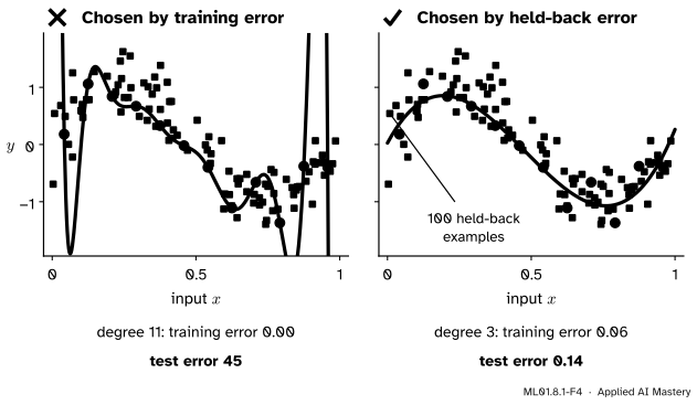
Wrong beside right. The training error picks the curve that threads every training point. The held-back examples pick the curve that follows the cloud.
“The model with the lowest training error is the best model.”
By Result 1 the training error never rises with the degree, so judged by it the highest degree on offer always wins, tied at worst. Choose with examples the fit has not seen. Once those examples have made a choice they are a validation set (lesson ML01.2.2), and the report needs a fresh test set.
“A flexible family contains the simple one, so it can only do better.”
It can represent everything the simple family can: the degree-9 family contains every cubic. But least squares does not pick the cubic from it. It picks whatever fits the twelve points best, and that member also fits their noise.
“Overfitting is a property of the model.”
It is a property of a model and a dataset. Degree 9 overfits twelve points. Given a hundred or more it does well, as lesson 3 shows. The question is never “is this model too flexible?” but “is it too flexible for the data I have?”
Check yourself
Recall
1. What is a polynomial model of degree \(d\), and how many parameters does it have?
Show answer
\(\hat{y} = {w_0 + w_1 x + \dots + w_d x^d}\), with \({d + 1}\) parameters. It is a linear model whose features are the powers of \(x\).
2. Why can the training error not rise when the degree is raised by one?
Show answer
Setting the new weight to zero gives back the old polynomial, so the larger family contains the smaller one, and its best member is at least as good.
3. Twelve training examples have twelve different inputs. From which degree on is the training error certain to be zero?
Show answer
From degree 11, which is \({n - 1}\): a polynomial of that degree passes through all twelve points.
4. How do underfitting and overfitting show up in the training error and the test error?
Show answer
Underfitting: both are high. Overfitting: the training error is low and the test error is much higher.
5. On the twelve points, which degree had the lowest test error, and what happened to the test error at degrees 10 and 11?
Show answer
Degree 3, with \(0.138\). At degrees 10 and 11 it was \(10.7\) and \(45\), while the training error fell to \(0\).
Exercises
1.★ The training set is \((0, 1)\), \((1, 3)\), \((2, 2)\). Find the best polynomial of degree 0 and its training error. Without any fitting, give the training error of the best polynomial of degree 2.
Show solution
Degree 0 is the mean, \({(1 + 3 + 2)/3} = 2\). Its misses are \(-1\), \(1\) and \(0\), so the training error is \({(1 + 1 + 0)/3} \approx 0.67\). There are three points with different inputs, so by Result 2 a polynomial of degree \({3 - 1} = 2\) passes through all of them: training error \(0\).
2.★★ Build the parabola through the three points of exercise 1 one point at a time, as in the worked example. The least-squares line through the same points is \(\hat{y} = {1.5 + 0.5x}\). A new example arrives: \((3, 2.5)\). Find the squared error of each model on it.
Show solution
Through \((0, 1)\): \(p = 1\). Through \((1, 3)\): add \(a\,x\) with \({1 + a} = 3\), so \(a = 2\). Through \((2, 2)\): add \({b\,x(x - 1)}\) with \({1 + 4 + 2b} = 2\), so \(b = -1.5\). The parabola is \(p(x) = {1 + 2x - {1.5\,x(x - 1)}}\).
At \(x = 3\) it predicts \({1 + 6 - {1.5 \cdot 6}} = -2\), a squared error of \({(-2 - 2.5)^2} = 20.25\). The line predicts \({1.5 + 1.5} = 3\), a squared error of \({(3 - 2.5)^2} = 0.25\). The model with zero training error is 81 times worse on the new example.
3.★★★ Show that the best parabola through the course’s four points is the line \(\hat{y} = {1.4x + 0.5}\) itself. Use the fact from lesson ML01.4.3 that weights are a least-squares solution exactly when the residuals are perpendicular to every column of the design matrix.
Show solution
The line’s residuals \({\hat{y} - y}\) at \(x = 1, 2, 3, 4\) are \(-0.1\), \(0.3\), \(-0.3\) and \(0.1\). They are already perpendicular to the column of ones and to the column \(x\), because the line is the least-squares line. The parabola adds one column, \(x^2 = (1, 4, 9, 16)\). Its dot product with the residuals is
So the weights \((0.5, 1.4, 0)\) make the residuals perpendicular to all three columns, which makes them the least-squares solution of degree 2. The extra weight is \(0\), and the training error stays at \(0.05\): Result 1 says it cannot rise, not that it must fall.
Summary card
Training error never punishes flexibility. Test error rewards it only up to a point.
ML01.8.1-F1
Too simple, about right, too flexible.
Polynomial of degree \(d\).\(\hat{y} = {w_0 + w_1 x + \dots + w_d x^d}\): a linear model on the powers of \(x\), with \({d + 1}\) weights.
Training error. Never rises with the degree. With \(n\) different inputs it is \(0\) from degree \({n - 1}\) on.
Underfitting. Both errors high. Overfitting. Training error low, test error much higher.
Twelve points. Test error \(0.32\) at degree 1, \(0.14\) at degree 3, \(0.70\) at degree 9, \(45\) at degree 11.
Sources and next steps
Sources. Each was opened and checked against this lesson on 12 November 2026.
Ian Goodfellow, Yoshua Bengio and Aaron Courville, Deep Learning, MIT Press, 2016, Section 5.2. Underfitting is failing to reach a low enough error on the training set, and overfitting is too large a gap between training and test error. Capacity is a model’s ability to fit a wide variety of functions. Equations 5.15 to 5.17 build polynomial regression by feeding powers of \(x\) to linear regression, and Figure 5.2 compares a linear, a quadratic and a degree-9 fit.
Aston Zhang, Zachary Lipton, Mu Li and Alexander Smola, Dive into Deep Learning, Section 3.6.2: higher-order polynomials always reach a training error that is lower or at worst equal, and a polynomial whose degree equals the number of examples can fit the training set perfectly (Result 2 shows that one degree less is enough).
scikit-learn 1.9.1 documentation, Underfitting vs. Overfitting. The same experiment with polynomial features of degree 1, 4 and 15 on a noisy cosine. Also LinearRegression: the parameter tol, default 1e-6, is passed as cond to scipy.linalg.lstsq on dense data from version 1.9.
NumPy 2.5 reference, Polynomial.fit. A least-squares fit to data, returned on a rescaled domain to reduce ill conditioning.
Next.ML01.8.2 Bias and variance asks what would happen if the twelve points were drawn again, and splits the test error into three parts.