Plot the training error and the validation error against the number of training examples. Where the two curves level off shows the bias, and the gap between them shows the variance. Derive the curve of the simplest model and learn to read the rest.
Build a learning curve: the training error and the validation error against the number of training examples.
Explain why the training error rises and the validation error falls as examples are added.
Tell high bias from high variance by the level and the gap of a learning curve.
Derive the learning curve of the mean model and check it by counting.
Read a complexity curve and say how the best degree moves as the training set grows.
In review. The maths and code on this page are checked by automated tests on every change, but an independent reader has not signed it off yet. Spot a mistake or a confusing step? Tell us.
The question
Your model’s error on new examples is too high. One colleague says: collect more data. Another says: build a bigger model. Both cost money, and one of them is a waste. Lesson 2 told bias from variance by redrawing the training set two thousand times. You have one training set. Which chart, made from the data you already have, settles the argument?
From the last lesson
1. Into which three parts does the expected squared error of a prediction split?
Show answer
Bias squared, variance and noise: the squared miss of the average fit, the scatter of the fits around their average, and the scatter of the targets around the truth.
2. As the degree of the polynomial rises, what happens to bias², variance and noise?
Show answer
Bias² falls, variance rises, the noise stays the same. Their sum falls and then rises.
Intuition
Train the same model on a small part of the data, then on a larger part, then on all of it. Each time, measure two errors: on the examples it was trained on, and on examples held back. Plot both against the number of training examples. That chart is a learning curve.
The held-back error now guides a decision, so by the rule of lesson ML01.2.2 it is a validation error, and its points are drawn as diamonds.
ML01.8.3-F1
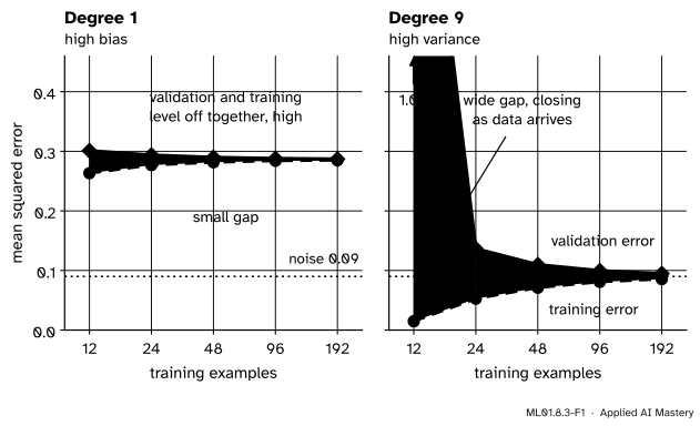
Two learning curves. For the line, the two errors level off together, high above the noise. For degree 9, they start far apart and close in on the noise level.
Two features of the chart carry the diagnosis.
The level the curves head for. If it is high, the model has high bias. More data only brings the curves to that level sooner.
The gap between the curves. If it is wide, the model has high variance. More data narrows it.
Build it up
Step 1. Make the curve. For each size \(n\), draw a training set of \(n\) examples from the source of lesson 1, at \(n\) evenly spaced inputs. Fit the model and record its training error and its validation error. Average over 2,000 training sets, so that the curve shows the pattern and not the luck of one draw.
\(n\)
Degree 1: training, validation
Degree 9: training, validation
12
\(0.263\), \(0.301\)
\(0.015\), \(0.996\)
24
\(0.277\), \(0.294\)
\(0.053\), \(0.136\)
48
\(0.282\), \(0.290\)
\(0.071\), \(0.110\)
96
\(0.284\), \(0.288\)
\(0.081\), \(0.100\)
192
\(0.285\), \(0.287\)
\(0.086\), \(0.095\)
Step 2. Why the training error rises. A few points are easy to fit: a line can pass exactly through any two points with different inputs. Each new point is one more demand on the same few weights, so the fit gets worse.
Step 3. Why the validation error falls. More points average more of the noise away, so the fit moves less from one training set to the next. That is variance shrinking.
Step 4. Where they meet. With endless data the variance is gone and both errors equal noise plus bias². For the line that is \({0.09 + 0.196} = 0.286\). For degree 9 it is \({0.09 + 0} = 0.09\). The line reached its level almost at once. Degree 9 needed about a hundred examples.
Step 5. The other curve. Lesson 1 plotted error against the degree for one training-set size. That is a complexity curve. Draw it for several sizes.
ML01.8.3-F2
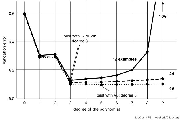
The complexity curve at three training-set sizes. More data flattens the right arm of the U, and the best degree moves from 3 to 5.
A flexible model that was reckless on 12 examples is safe on 96. More data buys the right to use a richer model.
The formal statement
NoteDefinition: learning curve, complexity curve
For one family of models, the learning curve is the pair of functions
\[
n \mapsto \closs{L_{\text{train}}}, \qquad n \mapsto \closs{L_{\text{val}}},
\]
where \(n\) is the number of training examples. The complexity curve shows the same two errors against a measure of flexibility, such as the degree, with \(n\) held fixed.
Result: the learning curve of the mean. Take the simplest model, which answers every question with the mean \(\bar{y}\) of its \(n\) training targets. Let the source be \(y = {\mu + \varepsilon}\): a constant truth, so that the model has no bias, plus noise of variance \(\sigma^2\). Then
where \(L_{\text{new}}\) is the squared error on a new example.
Step 1. The mean of \(n\) targets has variance \(\sigma^2/n\). The sum of \(n\) independent targets has variance \(n\sigma^2\), and dividing by \(n\) divides the variance by \(n^2\) (Facts A and B of lesson ML01.2.3).
Step 2. A new example. Its target \(y'\) is independent of \(\bar{y}\). By lesson 2, the expected squared error is bias² plus variance plus noise:
The sum in the third line is \({n\bar{y} - n\bar{y}} = 0\). Take the average of what is left. The left side has average \(n\sigma^2\), and the last term has average \({n \cdot \sigma^2/n} = \sigma^2\) by Step 1. So
Divide by \(n\) to get the expected training error, \({\sigma^2 (1 - 1/n)}\).
The training error starts below the noise and rises to it. The error on new examples starts above and falls to it. The gap between them is \(2\sigma^2/n\). These are the formulas that lesson ML01.2.3 found for one bin of a table, with \(n\) in place of the bin’s head count.
The general pattern. The mean has one parameter. A least-squares model with \(p\) parameters behaves the same way with \(p\) in place of \(1\). Average its squared bias over the training inputs, as lesson 2 averaged it over all inputs, and call that average \(\text{bias}^2\). Then
where the new examples sit at the training inputs with fresh noise. The block below proves it. Three readings follow.
Level. Both curves head for \({\text{bias}^2 + \sigma^2}\): noise plus bias².
Gap. It is \(2\sigma^2 p/n\). What matters is parameters per example.
Check. For degree 9, \(p = 10\) and \(\text{bias}^2\) is about \(0\). The formula gives a training error of \({0.09\,(1 - 10/n)}\): \(0.015\), \(0.053\), \(0.071\), \(0.081\) and \(0.085\) (the second is \(0.0525\) exactly), against the measured \(0.015\), \(0.053\), \(0.071\), \(0.081\) and \(0.086\).
The measured validation error at \(n = 12\) is far above the formula’s \(0.165\). Validation examples fall between and beyond the training inputs, where a flexible polynomial swings. From \(n = 48\) on the two agree.
Go deeper: proof for least squares with p parameters
Let \(\mat{X}\) be the \(n \times p\) design matrix, with independent columns. By lesson ML01.4.3 the fitted values are \(\mat{H}\vect{y}\), where \(\mat{H} = \mat{X}(\mat{X}\T\mat{X})^{-1}\mat{X}\T\). Three facts about \(\mat{H}\):
\(\mat{H}\T = \mat{H}\), because \(\mat{X}\T\mat{X}\) and its inverse are symmetric.
\(\mat{H}\mat{H} = \mat{H}\): the middle \(\mat{X}\T\mat{X}(\mat{X}\T\mat{X})^{-1}\) cancels.
The diagonal entries of \(\mat{H}\) add up to \(p\). For any two matrices, the diagonal of \(\mat{A}\mat{B}\) and of \(\mat{B}\mat{A}\) have the same sum, \(\sum_i \sum_j a_{ij} b_{ji}\). With \(\mat{A} = \mat{X}\) and \(\mat{B} = (\mat{X}\T\mat{X})^{-1}\mat{X}\T\), the product \(\mat{B}\mat{A}\) is the \(p \times p\) identity, whose diagonal adds up to \(p\).
Write the targets as \(\vect{y} = {\vect{f} + \vect{\varepsilon}}\), truth plus noise.
New examples. Fitted value \(i\) is \(\sum_j h_{ij} y_j\), so by lesson 2 its variance is \(\sigma^2 \sum_j h_{ij}^2\). Adding over \(i\) gives \(\sigma^2 \sum_i \sum_j h_{ij}^2\). That double sum is the diagonal sum of \(\mat{H}\mat{H}\T = \mat{H}\mat{H} = \mat{H}\), which is \(p\). So the average variance is \(\sigma^2 p/n\), and the expected error is that variance, plus the noise \(\sigma^2\), plus \(\text{bias}^2\).
Training examples. The residuals are \({(\mat{I} - \mat{H})\vect{f}} + {(\mat{I} - \mat{H})\vect{\varepsilon}}\). The first part is minus the bias at each training input, with squared length \({n \cdot \text{bias}^2}\). The second has mean zero, so the cross term averages to nothing, and its expected squared length is \(\sigma^2\) times the sum of the squared entries of \({\mat{I} - \mat{H}}\). That matrix is also symmetric and equal to its own square, so the sum is its diagonal sum, \({n - p}\). Dividing by \(n\) gives \(\text{bias}^2\) plus \({\sigma^2 (1 - p/n)}\).
Worked example
Work out the learning curve of the mean by hand, and check it by counting.
The source is the coin flip of lesson 2 around a constant truth: every target is \({3 + 2}\) or \({3 - 2}\), so \(\sigma^2 = 4\).
One training example. The model answers with that one target, so its training error is \(0\). A new target equals it half the time (error \(0\)) and differs by \(4\) half the time (error \(16\)): the expected error is \(8\). The formulas agree: \({4\,(1 - 1)} = 0\) and \({4\,(1 + 1)} = 8\).
Two training examples. There are four equally likely training sets. The last two columns are the training error and the expected error on a new example. With a mean of \(1\), a new target of \(1\) or \(5\) gives \({(0 + 16)/2} = 8\). With a mean of \(3\) it gives \({(4 + 4)/2} = 4\).
Targets
Mean
Training
New
\(1, 1\)
\(1\)
\(0\)
\(8\)
\(1, 5\)
\(3\)
\(4\)
\(4\)
\(5, 1\)
\(3\)
\(4\)
\(4\)
\(5, 5\)
\(5\)
\(0\)
\(8\)
The averages are \({(0 + 4 + 4 + 0)/4} = 2\) and \({(8 + 4 + 4 + 8)/4} = 6\). The formulas agree: \({4\,(1 - \tfrac12)} = 2\) and \({4\,(1 + \tfrac12)} = 6\).
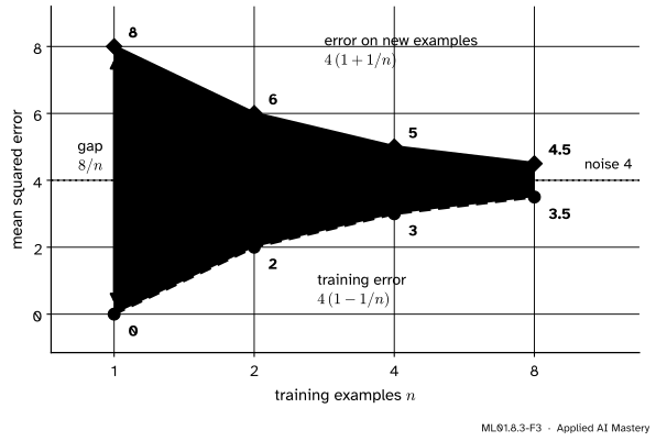
Four and eight. The formulas give \(3\) and \(5\), then \(3.5\) and \(4.5\).
ML01.8.3-F3
The learning curve of the mean, worked by hand. The two errors approach the noise, \(4\), from opposite sides, and the gap halves each time the data doubles.
Use it. How many examples bring the error on new examples within \(0.1\) of the noise? We need \(4/n \le 0.1\), so \(n \ge 40\).
Code
The worked example, by listing every possible training set.
from itertools import productfor n in (1, 2, 4, 8): # the mean of n targets, each 3 plus or minus 2 train, new = [], []for flips in product([-2, 2], repeat=n): # every possible training set targets = [3+ e for e in flips] mean =sum(targets) / n train.append(sum((t - mean) **2for t in targets) / n) new.append(sum((3+ e - mean) **2for e in (-2, 2)) /2)print(f"n = {n}: training error {sum(train) /len(train):.1f} "f"error on new examples {sum(new) /len(new):.1f} "f"formulas {4* (1-1/ n):.1f} and {4* (1+1/ n):.1f}")
n = 1: training error 0.0   error on new examples 8.0   formulas 0.0 and 8.0
n = 2: training error 2.0   error on new examples 6.0   formulas 2.0 and 6.0
n = 4: training error 3.0   error on new examples 5.0   formulas 3.0 and 5.0
n = 8: training error 3.5   error on new examples 4.5   formulas 3.5 and 4.5
Now the polynomials. Because we made the source, the validation error can be measured without luck: by lesson 2 it is the squared distance from the true curve, averaged over inputs, plus the noise.
import numpy as npdef true_curve(x):return np.sin(2* np.pi * x)def powers(x, degree):return np.column_stack([x ** k for k inrange(degree +1)])def inputs(n):return (np.arange(n) +0.5) / n # n evenly spaced inputs between 0 and 1sigma =0.3grid = inputs(200) # 200 inputs standing for "every input"def average_errors(degree, n, trials=2000, seed=0):"""Training and validation error of a polynomial, averaged over many training sets of size n.""" x = inputs(n) Y = true_curve(x)[:, None] + sigma * np.random.default_rng(seed).normal(size=(n, trials)) W, *_ = np.linalg.lstsq(powers(x, degree), Y, rcond=None) train = np.mean((powers(x, degree) @ W - Y) **2) validation = np.mean((powers(grid, degree) @ W - true_curve(grid)[:, None]) **2) + sigma **2return train, validationsizes = [12, 24, 48, 96, 192]curve = {degree: [average_errors(degree, n) for n in sizes] for degree in (1, 9)}for n, low, high inzip(sizes, curve[1], curve[9]):print(f"n = {n:3d} degree 1: training {low[0]:.3f}, validation {low[1]:.3f} "f"degree 9: training {high[0]:.3f}, validation {high[1]:.3f}")
n =  12   degree 1: training 0.263, validation 0.301   degree 9: training 0.015, validation 0.996
n =  24   degree 1: training 0.277, validation 0.294   degree 9: training 0.053, validation 0.136
n =  48   degree 1: training 0.282, validation 0.290   degree 9: training 0.071, validation 0.110
n =  96   degree 1: training 0.284, validation 0.288   degree 9: training 0.081, validation 0.100
n = 192   degree 1: training 0.285, validation 0.287   degree 9: training 0.086, validation 0.095
The complexity curve at three sizes.
for n in (12, 24, 96): validation = [average_errors(degree, n)[1] for degree inrange(10)]print(f"n = {n:2d} best degree {int(np.argmin(validation))} validation error by degree:"," ".join(f"{v:.2f}"for v in validation))
n = 12   best degree 3   validation error by degree: 0.60 0.30 0.31 0.13 0.14 0.14 0.16 0.20 0.33 1.00
n = 24   best degree 3   validation error by degree: 0.59 0.29 0.30 0.11 0.11 0.11 0.12 0.12 0.13 0.14
n = 96   best degree 5   validation error by degree: 0.59 0.29 0.29 0.10 0.10 0.10 0.10 0.10 0.10 0.10
In practice there is one dataset and no known truth. scikit-learn’s learning_curve holds part of the data back, trains on growing subsets of the rest, and repeats over many splits. Here it gets 300 examples at random inputs.
from sklearn.linear_model import LinearRegressionfrom sklearn.model_selection import ShuffleSplit, learning_curve, validation_curvefrom sklearn.pipeline import make_pipelinefrom sklearn.preprocessing import PolynomialFeaturesrng = np.random.default_rng(2)X = rng.uniform(0, 1, size=(300, 1)) # 300 examples at random inputsy = true_curve(X[:, 0]) + sigma * rng.normal(size=300)splits = ShuffleSplit(n_splits=50, test_size=60, random_state=0) # 50 ways to hold back 60 exampleslibrary = {}for degree in (1, 9): model = make_pipeline(PolynomialFeatures(degree), LinearRegression(tol=1e-12)) n_used, train_scores, val_scores = learning_curve( model, X, y, train_sizes=[24, 48, 96, 192], cv=splits, scoring="neg_mean_squared_error") library[degree] = (np.median(-train_scores, axis=1), np.median(-val_scores, axis=1), np.mean(-val_scores, axis=1))print(f"degree {degree} sizes {n_used} training {np.round(library[degree][0], 3)} "f"validation {np.round(library[degree][1], 3)}")model = make_pipeline(PolynomialFeatures(), LinearRegression(tol=1e-12))for m in (24, 240): # the complexity curve, on 24 and on 240 examples _, val_scores = validation_curve( model, X[:m], y[:m], param_name="polynomialfeatures__degree", param_range=list(range(1, 10)), scoring="neg_mean_squared_error", cv=ShuffleSplit(n_splits=50, test_size=0.2, random_state=0))print(f"{m} examples: best degree {int(np.argmin(np.median(-val_scores, axis=1))) +1}")
The scores are negative errors, because scikit-learn always maximises, and the numbers are medians over the 50 splits. The pattern is the one above: the line levels off near \(0.30\) with almost no gap, and degree 9 closes its gap and ends near the noise, \(0.09\). With 24 randomly placed examples a few of the 50 splits produce a degree-9 curve that shoots far off, and the mean validation error over the splits is above \(5\). Randomly placed inputs leave gaps, and a flexible curve swings in the gaps: on average its variance is larger than on evenly spaced inputs.
Explore
In the polynomial fitter of the previous lesson, set the degree to 9 and pile up fits with 12 points. Then switch to 48 points and pile up fits again: the fan of curves closes up.
Pitfalls
ML01.8.3-F4
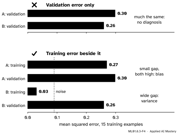
Wrong beside right. Model A is the line and model B is degree 9, each trained on 15 examples. Their validation errors look alike. Their training errors tell them apart.
“The validation error tells me what is wrong with the model.”
It tells you that something is wrong. Models A and B have nearly the same validation error and need opposite cures. The diagnosis needs the training error beside it.
“The training error should go down as I add data.”
It goes up, because more points are harder to fit. A rising training error on a learning curve is healthy. What should go down is the validation error.
“The two curves have met, so the model is good.”
They have met, so more data will not help. Whether the model is good depends on where they met. The line’s curves meet at \(0.29\), three times the noise. In machine learning this is the check to make before paying for more data.
Check yourself
Recall
1. What is plotted on a learning curve?
Show answer
The training error and the validation error of one model family, against the number of training examples.
2. As training examples are added, which way does each error usually move, and why?
Show answer
The training error rises, because more points are harder to fit. The validation error falls, because the variance shrinks.
3. What does a learning curve with high bias look like?
Show answer
Both errors level off early at a high value, with a small gap between them.
4. What does a learning curve with high variance look like?
Show answer
A low training error, a much higher validation error, and a wide gap that narrows as examples are added.
5. For the mean of \(n\) targets with noise variance \(\sigma^2\) and no bias, what are the expected training error and the expected error on a new example?
Show answer
\({\sigma^2 (1 - 1/n)}\) and \({\sigma^2 (1 + 1/n)}\). The gap is \(2\sigma^2/n\).
Exercises
1.★ A model has training error \(0.40\) and validation error \(0.44\) on 100 examples, and \(0.41\) and \(0.42\) on 1,000 examples. An error of \(0.20\) would be acceptable. What is wrong with the model, and will 10,000 examples help?
Show solution
High bias. The two errors are close together and have levelled off near \(0.41\), twice the acceptable error. More examples can only close the remaining gap of \(0.01\), so 10,000 examples will leave the validation error at about \(0.41\). The model needs to be richer.
2.★★ The mean model is used on a source with constant truth and noise variance \(9\). Find its expected training error and expected error on a new example with \(n = 3\). How many training examples make the gap smaller than \(0.5\)?
Show solution
With \(n = 3\): \({9\,(1 - \tfrac13)} = 6\) and \({9\,(1 + \tfrac13)} = 12\). The gap is \(2\sigma^2/n = 18/n\). It is below \(0.5\) when \(n > 36\), so from 37 examples on.
3.★★★ Using the general pattern for \(p\) parameters, show that \(p\) drops out of the average of the two expected errors, and say what that average equals. Then estimate, from the row \(n = 24\) of the table in Step 1, the level that the degree-1 and degree-9 curves head for.
The terms in \(p/n\) cancel. So noise plus bias², the level the curves head for, lies halfway between them at every \(n\).
From the row \(n = 24\): for degree 1, \({(0.277 + 0.294)/2} = 0.2855\), against \({0.09 + 0.196} = 0.286\). For degree 9, \({(0.053 + 0.136)/2} = 0.0945\), close to the noise, \(0.09\). It is a little high because validation examples between the training inputs cost more than the formula assumes.
Summary card
The level of a learning curve shows the bias. The gap shows the variance.
ML01.8.3-F1
High level: bias. Wide gap: variance.
Learning curve. Training error and validation error against the number of training examples \(n\).
The mean model.\(\E[L_{\text{train}}] = {\sigma^2 (1 - 1/n)}\) and \(\E[L_{\text{new}}] = {\sigma^2 (1 + 1/n)}\).
Least squares, \(p\) parameters. Level \({\text{bias}^2 + \sigma^2}\), gap \(2\sigma^2 p/n\).
More data narrows the gap and never lowers the level. It also moves the best degree up: 3 with 12 examples, 5 with 96.
Sources and next steps
Sources. Each was opened and checked against this lesson on 12 November 2026.
Ian Goodfellow, Yoshua Bengio and Aaron Courville, Deep Learning, MIT Press, 2016, Section 5.2. Figure 5.3 shows training and generalisation error against capacity, with the underfitting and overfitting regimes. Figure 5.4 shows the effect of training-set size: a fixed model’s training error rises because larger datasets are harder to fit, its test error falls, too little capacity levels off at a high error, and the optimal capacity grows with the training set.
Andrew Ng, Advice for applying machine learning, CS229 lecture slides, Stanford University. The slides “More on bias vs. variance” give the typical learning curves: for high variance, a test error still decreasing and a large gap between training and test error; for high bias, a training error that is itself unacceptably high and a small gap.
scikit-learn 1.9.1 User Guide, Section 3.5, Validation curves: plotting scores to evaluate models. A learning curve shows the validation and training score of an estimator for varying numbers of training samples. If both scores converge to a low value, more training data will probably not help. Also the API reference for learning_curve and validation_curve, whose scores have one column per split.