When a model predicts a number, each prediction misses by some amount. Compute the mean absolute error, the mean squared error, its root and R squared on one small test set, see which units each carries, how a single outlier moves them, and why each needs a baseline beside it.
Compute the mean absolute error, the mean squared error, the root mean squared error and R squared of a set of predictions by hand.
State the units of each metric and say how each changes when the target is measured in other units.
Show that the RMSE is never below the MAE, and say what a wide gap between them means.
Explain why one large miss moves the RMSE more than the MAE.
Compare a model with the baseline of always predicting the training mean, and read R squared as that comparison.
In review. The maths and code on this page are checked by automated tests on every change, but an independent reader has not signed it off yet. Spot a mistake or a confusing step? Tell us.
The question
A model predicts exam marks from hours of study, and a report says: “the error is 2 marks”. Two marks, measured how? As a typical miss, or in a way that punishes large misses more? And two marks compared with what? Would guessing the class average for everyone have done nearly as well?
From the last lesson
1. What does the AUC measure, as a probability?
Show answer
The probability that a randomly chosen positive has a higher score than a randomly chosen negative.
2. Where is the no-information line on a ROC plot, and where on a precision-recall plot?
Show answer
The diagonal on a ROC plot. A horizontal line at the share of positives on a precision-recall plot.
Intuition
A classifier’s answer is right or wrong. A regression model predicts a number, and almost every prediction is a little off: by how much?
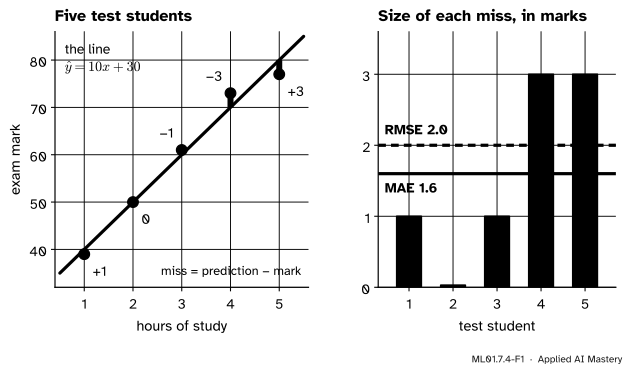
Here is a small invented case. A line fitted earlier to other students predicts an exam mark out of 100 from the hours of study: \({\hat{y} = 10x + 30}\). Five new students form the test set. For each one the error is the prediction minus the mark, \({e = \hat{y} - y}\), the quantity that module ML01.4 called the residual.
ML01.7.4-F1
The same five misses, summed up in two ways. The MAE is their mean size. The RMSE lies above it, because it gives the two misses of 3 marks more say.
Both summaries are in marks, and both say how far off the model typically is. They differ in the weight a large miss gets. The mean absolute error (MAE) treats every mark of error alike. The root mean squared error (RMSE) squares the errors first, so a miss of 3 counts nine times as much as a miss of 1.
Build it up
Step 1. The errors. At 1 to 5 hours the line predicts \({40, 50, 60, 70, 80}\). The marks were \({39, 50, 61, 73, 77}\). The errors are \({+1,\ 0,\ -1,\ -3,\ +3}\).
Step 2. MAE: average the sizes. Drop the signs and take the mean: \({(1 + 0 + 1 + 3 + 3)/5 = 1.6}\) marks.
Step 3. MSE: average the squares. Square each error and take the mean: \({(1 + 0 + 1 + 9 + 9)/5 = 4}\). This mean squared error is the loss of ML01.4. Its unit, marks squared, is hard to picture.
Step 4. RMSE: take the root.\({\sqrt{4} = 2}\) marks, back in the units of the target.
Step 5. The gap between them. The RMSE, \(2\), is above the MAE, \(1.6\). It always is, unless every miss has the same size. A wide gap means that a few misses are much larger than the rest.
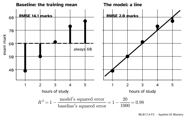
Step 6. A baseline. Is 2 marks good? Compare it with a model that ignores the hours. The students the line was fitted to had a mean mark of 60, so the simplest model says “60” for everyone.
ML01.7.4-F2
The same test students scored by two models. The baseline misses by 14.1 marks, the line by 2.
The line cuts the baseline’s RMSE of \(14.1\) marks to \(2\). R squared, met in lesson ML01.4.4, turns this comparison into one number with no units: the share of the baseline’s squared error that the model removes. Here it is \(0.98\).
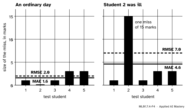
Step 7. One bad day. Suppose the second student was ill and scored 35, not 50. That one miss is now 15 marks.
ML01.7.4-F4
One changed mark. The MAE rises from 1.6 to 4.6 and the RMSE from 2 to 7.
The MAE nearly triples. The RMSE more than triples, and the MSE goes from \(4\) to \(49\): squaring lets one far-off example dominate the total.
The formal statement
NoteDefinition: four regression metrics
For \(n\) examples with targets \(y_i\), predictions \(\hat{y}_i\) and errors \({e_i = \hat{y}_i - y_i}\),
All four are computed on data the model was not fitted to (module ML01.2).
Result 1: units. With the target in marks, each error is in marks, and so is the MAE. Each squared error is in marks squared, so the MSE is too, and its root, the RMSE, is in marks again. In \(R^2\) one sum of squares is divided by another, so the units cancel.
Change the units by multiplying every target and every prediction by a number \(k\). Each error becomes \(k e_i\), with \({\abs{k e_i} = \abs{k}\,\abs{e_i}}\) and \({(k e_i)^2 = k^2 e_i^2}\), so
In \(R^2\) both sums are multiplied by \(k^2\), which cancels. So an MAE or an RMSE means nothing without its unit, and an MSE cannot be compared with either.
Result 2: the RMSE is never below the MAE. Write \({a_i = \abs{e_i}}\) for the size of miss \(i\) and \(m\) for the MAE, the mean of the sizes. Average the squared distances of the sizes from their mean. Expand the square, average each of its three terms, and use \({\frac{1}{n} \sum_i a_i^2 = \text{MSE}}\) and \({\frac{1}{n} \sum_i a_i = m}\):
The first line is a mean of squares, so it is never negative. Therefore \({\text{MSE} \ge \text{MAE}^2}\) and \({\text{RMSE} \ge \text{MAE}}\), with equality only when all the misses have the same size. In words: the MSE is the squared MAE plus the variance of the sizes of the misses.
Result 3: one large miss. Multiplying out \(\big(\sum_i \abs{e_i}\big)^2\) gives every \(e_i^2\) plus products \({\abs{e_i}\,\abs{e_j}}\) that are never negative. So the square of the sum is at least the sum of the squares, and
The upper end is reached when one example carries all the error. A single miss of size \(E\) among \({n - 1}\) perfect predictions gives an MAE of \(E/n\) and an RMSE of \(E/\sqrt{n}\). With \({n = 100}\) that miss shows up ten times larger in the RMSE than in the MAE.
Result 4: R squared is a comparison with a constant. A model that predicts \(\bar{y}\) for every example has an MSE of \({\frac{1}{n} \sum_i (y_i - \bar{y})^2}\). Divide the top and the bottom of the fraction in \(R^2\) by \(n\):
\[
R^2 = 1 - \frac{\text{MSE of the model}}{\text{MSE of predicting } \bar{y}} .
\]
\({R^2 = 1}\) means no error, \({R^2 = 0}\) means no better than that constant, and a negative \(R^2\) means worse, which can happen on test data.
Go deeper: which mean? the baseline you could really have used
The \(\bar{y}\) in \(R^2\) is the mean of the targets being scored. On a test set that is the test mean, which nobody knows when the predictions are made. The baseline you could actually use predicts the mean of the training targets.
Lesson ML01.4.1 showed that, of all constants, the mean of a set of numbers has the smallest mean squared error on those numbers. So the training mean can only tie with the test mean or do worse: its \(R^2\) is at most zero. On a random split the two means are close, so it is usually just below zero. In the code below it is \({-0.001}\) on real data.
The same lesson showed that the constant with the smallest mean absolute error is a median, so the natural baseline for the MAE is the training median.
Worked example
All four metrics for the five test students, by hand.
Mark \(y\)
Prediction \(\hat{y}\)
Error \(e\)
\(e^2\)
\(39\)
\(40\)
\(+1\)
\(1\)
\(50\)
\(50\)
\(0\)
\(0\)
\(61\)
\(60\)
\(-1\)
\(1\)
\(73\)
\(70\)
\(-3\)
\(9\)
\(77\)
\(80\)
\(+3\)
\(9\)
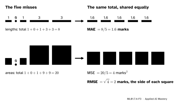
MAE. The sizes add up to \({1 + 0 + 1 + 3 + 3 = 8}\), so \({\text{MAE} = 8/5 = 1.6}\) marks.
MSE and RMSE. The squares add up to \({1 + 0 + 1 + 9 + 9 = 20}\), so \({\text{MSE} = 20/5 = 4}\) marks squared and \({\text{RMSE} = \sqrt{4} = 2}\) marks.
ML01.7.4-F3
A mean shares a total out equally. Share out the lengths and each is \(1.6\): the MAE. Share out the areas and each is a square of area \(4\) and side \(2\): the MSE and the RMSE.
Check Result 2. The sizes lie \({-0.6, -1.6, -0.6, 1.4, 1.4}\) from their mean of \(1.6\). The squares of those have mean \({7.2/5 = 1.44}\), and \({\text{MSE} - \text{MAE}^2 = 4 - 2.56 = 1.44}\).
R squared. The marks add up to \(300\), so \({\bar{y} = 60}\). Their distances from \(60\) are \({-21, -10, 1, 13, 17}\), with squares \({441 + 100 + 1 + 169 + 289 = 1000}\). So
\[
R^2 = 1 - \frac{20}{1000} = 0.98 .
\]
The baseline. “Always 60” has those distances as its errors, apart from the sign. Its MAE is \({(21 + 10 + 1 + 13 + 17)/5 = 12.4}\) marks, its MSE is \({1000/5 = 200}\) and its RMSE is \({\sqrt{200} = 14.1}\) marks. By Result 4, \({R^2 = 1 - 4/200 = 0.98}\) again.
With the outlier. The second mark becomes \(35\), so the errors are \({+1, +15, -1, -3, +3}\).
Ordinary day
One student ill
MAE
\(8/5 = 1.6\)
\(23/5 = 4.6\)
MSE
\(20/5 = 4\)
\(245/5 = 49\)
RMSE
\(2\)
\(7\)
The miss of 15 supplies \(15\) of the \(23\) marks of absolute error, about \(65\%\), and \(225\) of the \(245\) units of squared error, about \(92\%\). That is why the RMSE reacts more strongly. The new marks have mean \(57\) and squared distances \({324 + 484 + 16 + 256 + 400 = 1480}\), so \({R^2 = 1 - 245/1480 = 0.83}\).
Neither reaction is wrong. If one miss of 15 marks really is worse than five misses of 3, trust the RMSE. If the 35 is a fluke, the MAE gives the steadier picture.
Code
From scratch.
import numpy as npdef mae(y, y_hat):returnfloat(np.mean(np.abs(y_hat - y)))def mse(y, y_hat):returnfloat(np.mean((y_hat - y) **2))def rmse(y, y_hat):return mse(y, y_hat) **0.5def r_squared(y, y_hat):return1.0-float(np.sum((y_hat - y) **2) / np.sum((y - y.mean()) **2))hours = np.array([1.0, 2.0, 3.0, 4.0, 5.0])marks = np.array([39.0, 50.0, 61.0, 73.0, 77.0])line =10.0* hours +30.0# the model's predictionsalways_60 = np.full(5, 60.0) # the baseline: the training meanill = np.array([39.0, 35.0, 61.0, 73.0, 77.0]) # the second student has a bad dayprint("errors:", line - marks)for name, y, y_hat in [("the line", marks, line), ("always 60", marks, always_60), ("line, one ill", ill, line)]:print(f"{name:<14} MAE {mae(y, y_hat):5.2f} MSE {mse(y, y_hat):6.1f} RMSE {rmse(y, y_hat):5.2f} "f"R squared {r_squared(y, y_hat):5.2f}")share, of_line = marks /100, line /100# the same marks as fractions of 100print(f"in fractions of full marks: MAE {mae(share, of_line):.3f} MSE {mse(share, of_line):.4f} "f"RMSE {rmse(share, of_line):.2f} R squared {r_squared(share, of_line):.2f}")
errors: [ 1.  0. -1. -3.  3.]
the line       MAE  1.60  MSE    4.0  RMSE  2.00  R squared  0.98
always 60      MAE 12.40  MSE  200.0  RMSE 14.14  R squared  0.00
line, one ill  MAE  4.60  MSE   49.0  RMSE  7.00  R squared  0.83
in fractions of full marks: MAE 0.016  MSE 0.0004  RMSE 0.02  R squared 0.98
The last line shows Result 1: with marks as fractions of the full 100, the MAE and RMSE are divided by 100, the MSE by 10,000, and \(R^2\) stays \(0.98\).
The course’s four points and their least-squares line \({\hat{y} = 1.4x + 0.5}\) give the numbers of module ML01.4.
four points: MAE 0.200 MSE 0.050 RMSE 0.224 R squared 0.98
The library version, on scikit-learn’s diabetes dataset: 442 patients, 10 measurements each, and a target between 25 and 346 that measures how far the disease has progressed a year later. The split is that of lesson ML01.3.4. DummyRegressor always predicts the training mean.
from sklearn.datasets import load_diabetesfrom sklearn.dummy import DummyRegressorfrom sklearn.linear_model import LinearRegressionfrom sklearn.metrics import mean_absolute_error, mean_squared_error, r2_score, root_mean_squared_errorfrom sklearn.model_selection import train_test_splitdata = load_diabetes(scaled=False)X_train, X_test, y_train, y_test = train_test_split(data.data, data.target, test_size=0.2, random_state=0)models = {"a fitted line": LinearRegression(), "training mean": DummyRegressor(strategy="mean")}for name, model in models.items(): y_hat = model.fit(X_train, y_train).predict(X_test)print(f"{name:<14} MAE {mean_absolute_error(y_test, y_hat):5.1f} MSE {mean_squared_error(y_test, y_hat):6.0f} "f"RMSE {root_mean_squared_error(y_test, y_hat):5.1f} R squared {r2_score(y_test, y_hat):6.3f}")print(f"training mean {y_train.mean():.1f}, test mean {y_test.mean():.1f}")
a fitted line  MAE  46.2  MSE   3424  RMSE  58.5  R squared  0.332
training mean  MAE  59.2  MSE   5135  RMSE  71.7  R squared -0.001
training mean 151.6, test mean 154.2
The line’s RMSE of \(58.5\) means little alone. Beside the baseline’s \(71.7\) it says that the ten measurements remove only part of the error: \({R^2 = 0.332}\). The RMSE is about a quarter above the MAE, \(46.2\), so the misses vary in size. And the baseline’s own \(R^2\) is \({-0.001}\), not \(0\), because the training mean, \(151.6\), is not quite the test mean, \(154.2\).
Explore
This module’s interactive, in lesson 3, is about classification. For the metrics of this lesson, go back to the line fitter of lesson ML01.4.1. Its read-out gives the MSE and the MAE of your line. Drag one point far above the others, leave the line where it is, and compare how much each number grows.
Pitfalls
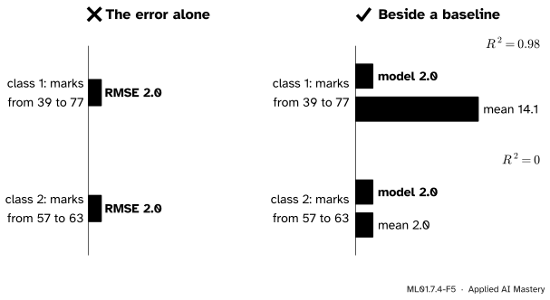
ML01.7.4-F5
Wrong beside right. The same RMSE of 2 marks is excellent where marks range from 39 to 77, and worthless where they range from 57 to 63, because there the mean does just as well.
“The RMSE is 2, so the model is good.”
Good compared with what? An error is small or large only beside the spread of the target. Report the same metric for a baseline, such as always predicting the training mean, or report \(R^2\), which makes that comparison for you. Every result in machine learning needs a baseline.
“The MSE is 4 and the MAE is 1.6, so the MSE is worse.”
They are in different units, marks squared and marks, and cannot be compared. Compare the RMSE with the MAE.
“MAE and RMSE always agree about which model is better.”
Take two models on five students. One misses by 2 marks every time. The other is exact four times and misses once by 9. The MAEs are \(2\) and \({9/5 = 1.8}\): the second model wins. The RMSEs are \(2\) and \({\sqrt{81/5} = 4.02}\): the first wins. Whether one large miss is worse than several small ones is for you to decide, not the metric.
Check yourself
Recall
1. Write the MAE, the MSE and the RMSE in terms of the errors \(e_i\).
2. The target is in marks. What are the units of the MAE, the MSE, the RMSE and \(R^2\)?
Show answer
Marks, marks squared, marks, and no units.
3. Which is larger, the MAE or the RMSE, and when are they equal?
Show answer
The RMSE is never smaller than the MAE. They are equal only when every miss has the same size.
4. Which of the two reacts more strongly to one large miss, and why?
Show answer
The RMSE, because the errors are squared before they are averaged, so a large miss takes a larger share of the total.
5. What do \({R^2 = 0}\) and a negative \(R^2\) say about a model?
Show answer
\({R^2 = 0}\): its squared error equals that of always predicting the mean of the targets. Negative: it is worse than that constant.
Exercises
1.★ A model predicts the prices of four flats, in thousands, as \({210, 150, 300, 240}\). The true prices are \({200, 160, 300, 270}\). Compute the MAE, the MSE and the RMSE, with their units.
Show solution
The errors are \({210 - 200 = 10}\), \({150 - 160 = -10}\), \(0\) and \({240 - 270 = -30}\).
The RMSE is above the MAE because one miss is much larger than the others.
2.★★ A second class sat an easy quiz. The marks of five test students were \({57, 63, 59, 61, 60}\), and a model predicted \({58, 62, 62, 58, 60}\). Compute the model’s RMSE, the RMSE of always predicting 60, and \(R^2\). Compare with the worked example.
Show solution
The errors are \({58 - 57 = 1}\), \({62 - 63 = -1}\), \({62 - 59 = 3}\), \({58 - 61 = -3}\) and \(0\). Their squares add up to \({1 + 1 + 9 + 9 + 0 = 20}\), so \({\text{MSE} = 4}\) and \({\text{RMSE} = 2}\) marks.
Always 60 has errors \({3, -3, 1, -1, 0}\), with the same squares in another order: its RMSE is also \(2\) marks. The mean of the marks is \({300/5 = 60}\), so \({R^2 = 1 - 20/20 = 0}\).
The RMSE is 2 marks, as in the worked example. But there the baseline was at \(14.1\) and \(R^2\) was \(0.98\); here the model is no better than saying “60” every time. The error alone cannot tell the cases apart.
3.★★★ A test set has \(n\) examples. A model is exact on \({n - 1}\) of them and misses the last by \(E\). (a) Find its MAE and RMSE and their ratio. (b) For \({E = 15}\), how large is each when \({n = 5}\) and when \({n = 500}\)? (c) Which bound of Result 3 does this case sit on?
Show solution
(a) \(\text{MAE} = \frac{1}{n}(0 + \dots + 0 + E) = \frac{E}{n}\). \({\text{MSE} = \frac{E^2}{n}}\), so \({\text{RMSE} = \frac{E}{\sqrt{n}}}\). The ratio is
(b) \({n = 5}\): \({\text{MAE} = 3}\) and \({\text{RMSE} = 15/\sqrt{5} = 6.71}\). \({n = 500}\): \({\text{MAE} = 0.03}\) and \({\text{RMSE} = 15/\sqrt{500} = 0.67}\). More data shrinks both, but the MAE shrinks like \(1/n\) and the RMSE only like \(1/\sqrt{n}\).
(c) The upper one: \({\text{RMSE} = \sqrt{n} \cdot \text{MAE}}\). One lone miss is the most uneven a set of errors can be.
Summary card
Average the sizes of the misses, or average their squares and take the root. Then set the result beside a baseline.
ML01.7.4-F1
Five misses, two summaries.
MAE.\(\frac{1}{n} \sum_i \abs{e_i}\), in the units of the target.
MSE and RMSE.\(\frac{1}{n} \sum_i e_i^2\), in squared units, and its root, in the units of the target.
Ordering.\({\text{MAE} \le \text{RMSE}} \le {\sqrt{n} \cdot \text{MAE}}\). A wide gap means uneven misses.
R squared.\(1 - \frac{\text{MSE of the model}}{\text{MSE of the mean}}\): no units, \(0\) for the mean, negative if worse.
Five marks. MAE \(1.6\), MSE \(4\), RMSE \(2\), \({R^2 = 0.98}\). With one miss of 15: MAE \(4.6\), RMSE \(7\).
Sources and next steps
Sources. Each was opened and checked against this lesson on 12 November 2026.
scikit-learn 1.9 User Guide, Metrics and scoring. Section 3.4.6.1 defines \(R^2\), and says that the best score is 1.0, that it can be negative, and that a constant model which always predicts the average of \(y\) scores 0.0. Sections 3.4.6.2 and 3.4.6.3 define the MAE and the MSE and describe the RMSE as a measure in the units of the target. Section 3.4.8 presents DummyRegressor, with its mean and median strategies, as a sanity check.
Rob J. Hyndman and George Athanasopoulos, Forecasting: Principles and Practice, 3rd edition, OTexts, Section 5.8. Defines the MAE and the RMSE on the scale of the data, and states that minimising the MAE leads to forecasts of the median and minimising the RMSE to forecasts of the mean.
scikit-learn 1.9 documentation, load_diabetes: 442 samples, 10 features, integer targets from 25 to 346. User Guide Section 9.1.2: the target measures disease progression one year after baseline.
Next. Module ML01.8, Overfitting, bias and variance, uses these metrics on training and test data side by side, to see when a model has learned the pattern and when it has learned the noise.