A feature measured in large units dominates a distance, so k-nearest neighbours can end up ignoring every other feature. Standardise each feature with the training mean and standard deviation, watch the nearest neighbour change, and meet Manhattan distance.
Show with numbers why the feature with the largest spread dominates Euclidean distance.
Standardise a feature by hand with the mean and standard deviation of the training set, and apply the same two numbers to a new example.
Prove that distances between standardised examples do not depend on the units a feature was recorded in.
Compute Manhattan distance and say how it differs from Euclidean distance.
Build a scikit-learn pipeline that scales and classifies without using the test rows to set the scale.
In review. The maths and code on this page are checked by automated tests on every change, but an independent reader has not signed it off yet. Spot a mistake or a confusing step? Tell us.
The question
Weigh a fruit in grams and measure its width in centimetres. Its nearest neighbour on the tray is a pear. Now write the same weights in kilograms and change nothing else. Its nearest neighbour is an apple. How can a prediction depend on the units someone chose, and what should “nearest” mean when the features measure different things?
From the last lesson
1. How does the \(k\)-nearest-neighbour classifier label a query?
Show answer
It finds the \(k\) stored examples closest to the query and predicts the label with the most votes among them.
2. Which set of examples chooses \(k\), and why not the training set?
Show answer
A validation set. Without duplicated inputs, the training error is \(0\) at \({k = 1}\) however noisy the labels, so the training set never prefers a larger \(k\).
Intuition
A distance adds up squared differences, one per feature. It does not know what the numbers mean. It adds a difference in grams to a difference in centimetres as though one gram and one centimetre were the same size of step.
They are not. Fruit on a tray differ in weight by tens of grams and in width by a centimetre or two, so the weight differences are the big numbers and the width hardly registers.
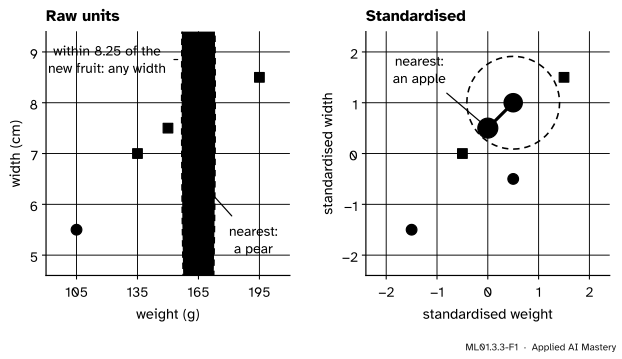
ML01.3.3-F1
A neighbourhood of the new fruit that holds exactly one stored fruit. Left: in grams and centimetres it is a circle of radius \(8.25\), but \(8.25\) cm is more than the whole range of widths, so on the page it is a band: only weight matters. Right: after standardising, the neighbourhood is a circle on the page too, and the nearest neighbour is a different fruit.
The fix is to give every feature the same ruler before measuring: its own spread, how far its values typically lie from their mean.
Build it up
Step 1. Look inside one distance. The new fruit weighs 165 g and is 8.0 cm wide. A stored apple weighs 150 g and is 7.5 cm wide. The differences are \(15\) g and \(0.5\) cm, and the squared distance is
\[
15^2 + 0.5^2 = 225 + 0.25 = 225.25 .
\]
The weight contributes \(225\) of the \(225.25\). That is \(99.9\%\).
Step 2. So the raw distance is nearly the weight difference. The distance is \({\sqrt{225.25} \approx 15.01}\), and the weight difference alone is \(15\).
Step 3. Change the unit and the roles swap. In kilograms the same weight difference is \(0.015\). The squared distance becomes \({0.015^2 + 0.5^2} = {0.000225 + 0.25}\), and now the width contributes \(99.9\%\). The distance obeys whichever feature has the larger numbers.
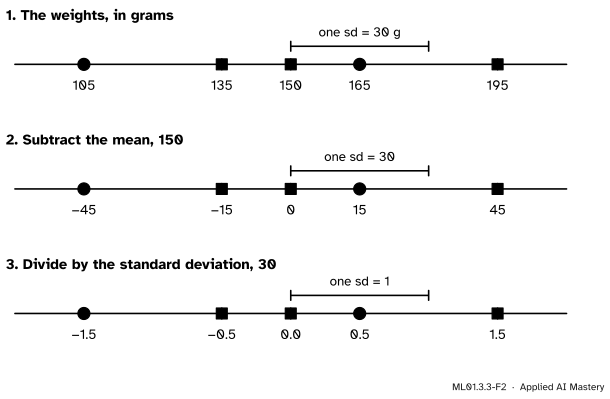
Step 4. Give each feature its own ruler. Take one feature’s values in the training set. Subtract their mean, so that they are centred on zero. Then divide by their standard deviation, so that a typical distance from the centre becomes \(1\). This is standardising, and the result is called a z-score.
ML01.3.3-F2
Standardising the five weights. The marks never move: only the ruler under them changes. On line 3 the ruler reads “standard deviations from the mean”.
Step 5. Use the training set’s ruler for everything. The mean and the standard deviation are worked out once, from the training examples. A new fruit is put on that same ruler. It does not get one of its own.
The formal statement
NoteDefinition: standardising a feature
Let feature \(j\) take the values \({x_{1j}, \dots, x_{nj}}\) in the training set. Its mean and standard deviation are
The two numbers per feature come from the training set alone. (The standard deviation here divides by \(n\), as scikit-learn’s StandardScaler does.)
Fact 1: a standardised training feature has mean 0 and standard deviation 1. Drop the index \(j\) and write \({z_i = (x_i - \mu) / \sigma}\). The mean of the \(z_i\) is
Standardising divides each feature’s difference by that feature’s spread before squaring. A difference of \(15\) g where the spread is \(30\) g counts as \(0.5\), and so does a difference of \(0.5\) cm where the spread is \(1\) cm.
Fact 3: the units no longer matter. Record feature \(j\) in a different unit, so that every value is multiplied by a constant \({c > 0}\) (for grams to kilograms, \({c = 0.001}\)). The new mean is
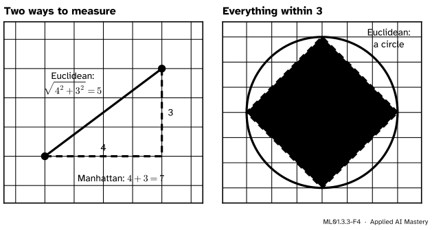
It is the length of a route that may only run along the axes, like a walk through a city of square blocks. Euclidean distance is the length of the straight route.
ML01.3.3-F4
Left: the same two points are \(5\) apart in a straight line and \(7\) apart along the grid. Right: the points within distance \(3\) of a centre form a circle for Euclidean distance and a diamond for Manhattan distance.
Squaring makes one large difference count for much more than several small ones. Manhattan distance does not square, so a single feature that is far out pulls it less. Which of the two predicts better is a question for the validation set, like \(k\). In scikit-learn the choice is the parameter p: p=2, the default, is Euclidean and p=1 is Manhattan. Manhattan distance adds grams to centimetres too, so it needs standardised features just as much.
Go deeper: Manhattan distance is never the shorter of the two
Write \({\Delta_j = \abs{a_j - b_j}}\), so that \({\operatorname{dist}_1 = \sum_j \Delta_j}\) and the Euclidean distance is \({\operatorname{dist} = \sqrt{\sum_j \Delta_j^2}}\). Square the Manhattan distance:
The extra terms are products of numbers that are not negative, so \({\operatorname{dist}_1 \ge \operatorname{dist}}\). The two are equal only when every cross term is zero, which means the points differ in at most one feature. That is why the diamond sits inside the circle and touches it only on the axes.
Worked example
Find the nearest neighbour of the fruit weighing 165 g and 8.0 cm wide, before and after standardising.
The tray holds five fruit.
Step 1: distances in raw units. Subtract the query, \({(165,\ 8.0)}\), square and add.
Fruit (g, cm)
Squared distance
Distance
pear \({(105, 5.5)}\)
\({60^2 + 2.5^2} = 3606.25\)
\(60.05\)
pear \({(165, 6.5)}\)
\({0^2 + 1.5^2} = 2.25\)
\(1.50\)
apple \({(135, 7.0)}\)
\({30^2 + 1^2} = 901\)
\(30.02\)
apple \({(150, 7.5)}\)
\({15^2 + 0.5^2} = 225.25\)
\(15.01\)
apple \({(195, 8.5)}\)
\({30^2 + 0.5^2} = 900.25\)
\(30.00\)
The nearest is the pear that weighs the same as the query, \(1.5\) away. The distances are nearly the weight differences \({60, 0, 30, 15, 30}\).
Step 2: the two rulers. The weights are \({105, 165, 135, 150, 195}\). Their sum is \(750\), so \({\mu = 150}\). The deviations from the mean are \({-45, 15, -15, 0, 45}\), with squares \({2025, 225, 225, 0, 2025}\), which add to \(4500\). So \({\sigma = \sqrt{4500 / 5}} = {\sqrt{900}} = 30\).
The widths are \({5.5, 6.5, 7.0, 7.5, 8.5}\). Their sum is \(35\), so \({\mu = 7}\). The deviations are \({-1.5, -0.5, 0, 0.5, 1.5}\), with squares \({2.25, 0.25, 0, 0.25, 2.25}\), which add to \(5\). So \({\sigma = \sqrt{5 / 5} = 1}\).
Step 3: distances on the rulers. Standardise every fruit, the new one included. The query becomes \(z = {\big( \tfrac{165 - 150}{30}, \tfrac{8.0 - 7}{1} \big)} = {(0.5,\ 1.0)}\).
Fruit, standardised
Squared distance
Distance
pear \({(-1.5, -1.5)}\)
\(2^2 + 2.5^2 = 10.25\)
\(3.20\)
pear \({(0.5, -0.5)}\)
\(0^2 + 1.5^2 = 2.25\)
\(1.50\)
apple \({(-0.5, 0)}\)
\(1^2 + 1^2 = 2\)
\(1.41\)
apple \({(0, 0.5)}\)
\(0.5^2 + 0.5^2 = 0.5\)
\(0.71\)
apple \({(1.5, 1.5)}\)
\(1^2 + 0.5^2 = 1.25\)
\(1.12\)
Now the nearest neighbour is the apple at \({(150\ \text{g},\ 7.5\ \text{cm})}\), at distance \(0.71\), and the next two are apples as well. The pear that was first is fourth.
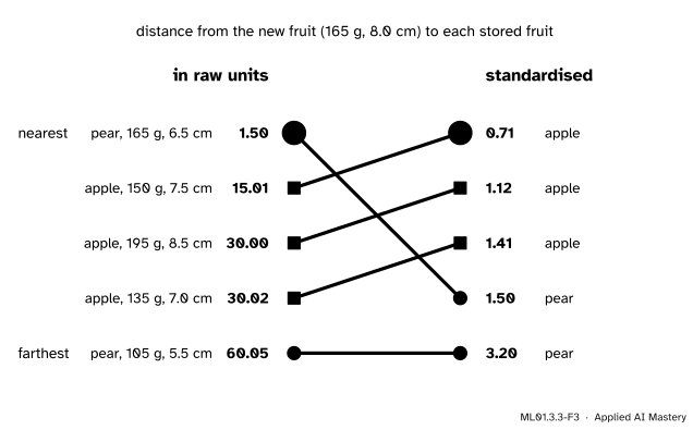
ML01.3.3-F3
The same five fruit ranked twice. In raw units the order is the order of weight differences. Standardised, the three apples move up and the pear drops from first to fourth.
The new fruit is \(8\) cm wide, wider than either pear. The standardised answer uses that. The raw answer could not see it.
Code
From scratch: the raw distances, then the same fruit with the weights in kilograms.
import numpy as npX = np.array([[105, 5.5], [165, 6.5], [135, 7.0], [150, 7.5], [195, 8.5]]) # weight (g), width (cm)y = np.array(["pear", "pear", "apple", "apple", "apple"])query = np.array([165, 8.0])def euclidean_to_all(X, query):return np.sqrt(((X - query) **2).sum(axis=1))raw = euclidean_to_all(X, query)print("grams: ", raw.round(2), "-> nearest is a", y[np.argmin(raw)])to_kg = np.array([0.001, 1.0]) # change the unit of the first feature onlyin_kg = euclidean_to_all(X * to_kg, query * to_kg)print("kilograms: ", in_kg.round(2), "-> nearest is an", y[np.argmin(in_kg)])weight_share = (150-165) **2/ ((150-165) **2+ (7.5-8.0) **2)print(f"share of the squared distance to the apple (150, 7.5) that comes from weight: {weight_share:.1%}")
grams:       [60.05  1.5  30.02 15.01 30.  ] -> nearest is a pear
kilograms:   [2.5 1.5 1.  0.5 0.5] -> nearest is an apple
share of the squared distance to the apple (150, 7.5) that comes from weight: 99.9%
The unit decided the answer. Now standardise with the mean and standard deviation of the stored fruit, and put the query on the same two rulers.
mean, sd = X.mean(axis=0), X.std(axis=0) # one pair of numbers per featureZ = (X - mean) / sdz_query = (query - mean) / sd # the query uses the tray's mean and sdstandardised = euclidean_to_all(Z, z_query)print("mean:", mean, " sd:", sd)print("standardised fruit:", Z.tolist())print("standardised query:", z_query)print("distances:", standardised.round(2), "-> nearest is an", y[np.argmin(standardised)])mean_kg, sd_kg = (X * to_kg).mean(axis=0), (X * to_kg).std(axis=0)print("same z-scores from kilograms:", np.allclose((X * to_kg - mean_kg) / sd_kg, Z))manhattan = np.abs(Z - z_query).sum(axis=1)print("Manhattan distances:", manhattan, "-> nearest is an", y[np.argmin(manhattan)])
mean: [150.   7.]  sd: [30.  1.]
standardised fruit: [[-1.5, -1.5], [0.5, -0.5], [-0.5, 0.0], [0.0, 0.5], [1.5, 1.5]]
standardised query: [0.5 1. ]
distances: [3.2  1.5  1.41 0.71 1.12] -> nearest is an apple
same z-scores from kilograms: True
Manhattan distances: [4.5 1.5 2.  1.  1.5] -> nearest is an apple
The numbers are those of the worked example, and kilograms give the same z-scores as grams (Fact 3). In scikit-learn, StandardScaler learns the mean and standard deviation in fit and applies them in transform. Chaining it to the classifier in a pipeline guarantees that both steps see the same training rows.
Five made-up fruit prove nothing about real data, so here is a real case: scikit-learn’s wine dataset, 178 wines in three classes, each described by 13 chemical measurements. One of them, proline, is recorded in the hundreds and thousands, and is spread far more widely than any other feature.
from sklearn.datasets import load_winefrom sklearn.model_selection import train_test_splitwine = load_wine()X_train, X_test, y_train, y_test = train_test_split(wine.data, wine.target, test_size=0.3, random_state=0, stratify=wine.target)spread =dict(zip(wine.feature_names, X_train.std(axis=0)))print(f"{len(X_train)} training wines, {len(X_test)} test wines, {wine.data.shape[1]} features")print(f"sd of proline: {spread['proline']:.0f} magnesium: {spread['magnesium']:.1f} hue: {spread['hue']:.2f}")squared = (X_test[:, None, :] - X_train[None, :, :]) **2# test wine, training wine, featureprint(f"share of all squared raw distance that comes from proline: {squared[:, :, 12].sum() / squared.sum():.1%}")models = {"raw units, 13 features": KNeighborsClassifier(n_neighbors=5),"standardised, Euclidean": make_pipeline(StandardScaler(), KNeighborsClassifier(n_neighbors=5)),"standardised, Manhattan": make_pipeline(StandardScaler(), KNeighborsClassifier(n_neighbors=5, p=1)),}scores = {name: model.fit(X_train, y_train).score(X_test, y_test) for name, model in models.items()}# Many wines share a proline value, so on proline alone distances tie and this score can move by a wine or two.proline_only = KNeighborsClassifier(n_neighbors=5).fit(X_train[:, [12]], y_train).score(X_test[:, [12]], y_test)print(f"proline alone, raw units: {proline_only:.2f}")for name, score in scores.items():print(f"{name}: {score:.3f}")
124 training wines, 54 test wines, 13 features
sd of proline: 325   magnesium: 14.1   hue: 0.22
share of all squared raw distance that comes from proline: 99.8%
proline alone, raw units: 0.61
raw units, 13 features: 0.722
standardised, Euclidean: 0.963
standardised, Manhattan: 0.981
On raw units the classifier gets \(39\) of the \(54\) test wines right, an accuracy of \(0.722\). Proline supplies \(99.8\%\) of the squared distance, so the other twelve measurements barely count: proline alone already scores about \(0.6\). With every feature standardised the same classifier gets \(52\) of \(54\), or \(0.963\). Only the rulers changed. Manhattan distance gets one more wine right: too small a difference to prefer it, and the test set is not the place to choose.
Explore
Go back to the neighbour explorer in lesson 2. Put the query at \({(6, 8)}\) on the fruit tray with \({k = 1}\), and move the slider “width counts” up to \({\times 10}\), as if widths were in millimetres. The neighbourhood becomes tall and thin, and the nearest neighbour jumps from the apple beside the query to the pear directly above it. Then switch to Manhattan distance and watch the neighbourhood turn into a diamond.
Pitfalls
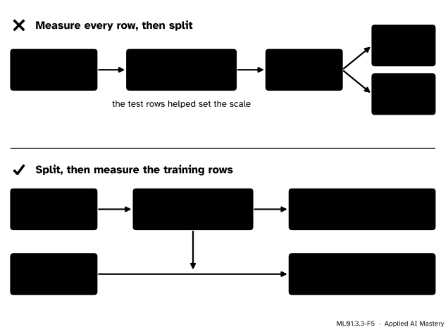
ML01.3.3-F5
Wrong beside right. The mean and the standard deviation are learned from the training rows only. The test rows, and every later example, are rescaled with those same two numbers.
“Standardise the whole table first, then split it.”
Then the test rows helped to set the mean and the standard deviation: information has leaked from the test set, as in lesson ML01.2.4. The score may hardly move, but it is no longer an honest estimate. Split first. A pipeline does it for you: its fit sees only the training rows.
“Standardise the test set with its own mean and standard deviation.”
Then training and test fruit are on different rulers, and a distance between them means nothing. The clearest case is a single new fruit: its mean is itself and its standard deviation is \(0\), so its “own” z-score is \({0 / 0}\). Use transform, never fit_transform, on anything that is not training data.
“After standardising, every feature matters the right amount.”
Every feature matters the same amount, which is different. A feature that has nothing to do with the label now has as much say as the most useful one, and its noise goes into every distance. Standardising is the sensible default. It does not replace thinking about which features belong in the table.
Check yourself
Recall
1. Why does a feature recorded in large numbers dominate Euclidean distance?
Show answer
The distance adds squared differences across features whatever their units, so the feature with the largest differences supplies almost all of the sum.
2. How is a feature standardised, and where do the two numbers come from?
Show answer
\({z = (x - \mu) / \sigma}\), with the mean \(\mu\) and the standard deviation \(\sigma\) computed from the training set only.
3. What are the mean and standard deviation of a training feature after standardising?
Show answer
Mean \(0\) and standard deviation \(1\).
4. Define Manhattan distance. How far apart are two points that differ by \(4\) in one feature and \(3\) in another?
Show answer
\({\operatorname{dist}_1(\vect{a}, \vect{b})} = {\sum_j \abs{a_j - b_j}}\), here \({4 + 3 = 7}\). The Euclidean distance is \({\sqrt{16 + 9} = 5}\).
5. Why is a new example never standardised with its own statistics?
Show answer
It must sit on the same ruler as the stored examples, and a single example has no spread: its standard deviation is \(0\).
Exercises
1.★ A feature takes the values \({2, 4, 4, 4, 5, 5, 7, 9}\) in the training set. Standardise the value \(9\), and a new value \(6\).
Show solution
The sum is \(40\), so \({\mu = 5}\). The deviations are \(-3, -1, -1, -1, 0, 0, 2, 4\), with squares \({9, 1, 1, 1, 0, 0, 4, 16}\), which add to \(32\). So \({\sigma = \sqrt{32 / 8} = 2}\). For \(9\): \({z = (9 - 5) / 2 = 2}\). For the new value \(6\): \({z = (6 - 5) / 2 = 0.5}\), with the same \(\mu\) and \(\sigma\).
2.★★ Use the standardised fruit of the worked example and the standardised query \({(0.5, 1.0)}\). (a) Compute the Manhattan distance to each fruit and name the nearest. (b) Two fruit tie for second place. What does that mean for \({k = 2}\)?
Show solution
(a) Add the absolute differences: pear \({(-1.5, -1.5)}\): \({2 + 2.5 = 4.5}\); pear \({(0.5, -0.5)}\): \({0 + 1.5 = 1.5}\); apple \({(-0.5, 0)}\): \({1 + 1 = 2}\); apple \({(0, 0.5)}\): \({0.5 + 0.5 = 1}\); apple \({(1.5, 1.5)}\): \({1 + 0.5 = 1.5}\). The nearest is the apple at \({(0, 0.5)}\), as with Euclidean distance.
(b) A pear and an apple are both at \(1.5\). With \({k = 2}\) only one of them can be the second neighbour, so the vote is either two apples or a one-all tie. This is the tied distance of lesson 2: the vote depends on the order in which the fruit were stored.
3.★★★Min-max scaling is \(x' = {(x - \min) / (\max - \min)}\), with the minimum and maximum taken from the training set. (a) Apply it to the five weights. (b) Show that it too gives the same result in any unit. (c) A sixth fruit weighing \(1005\) g is added. What happens to the scaled weights of the first five?
Show solution
(a) \({x' = (x - 105) / 90}\), so \({105, 165, 135, 150, 195}\) become \(0,\ 0.667,\ 0.333,\ 0.5,\ 1\).
(c) Now \({x' = (x - 105) / 900}\), and the five weights become \(0,\ 0.067,\ 0.033,\ 0.05,\ 0.1\), squeezed into a tenth of the range. Weight has almost dropped out of the distance, because one unusual value set the ruler. Standardising suffers too: the outlier enlarges \(\sigma\) from \(30\) to about \(320\).
Summary card
Give every feature the same ruler before you measure a distance.
ML01.3.3-F1
A band becomes a circle.
The problem. The feature with the largest numbers dominates: \({15^2 + 0.5^2 = 225.25}\) is \(99.9\%\) weight.
Standardise.\({z_j = (x_j - \mu_j) / \sigma_j}\), with \(\mu_j\) and \(\sigma_j\) from the training set only. Mean \(0\), standard deviation \(1\).
Effect on distance.\({\sum_j (a_j - b_j)^2 / \sigma_j^2}\). Changing a feature’s unit changes nothing.
Manhattan distance.\({\operatorname{dist}_1(\vect{a}, \vect{b})} = {\sum_j \abs{a_j - b_j}}\): differences \(4\) and \(3\) give \(7\), not \(5\).
In practice.make_pipeline(StandardScaler(), KNeighborsClassifier()), fitted on the training rows.
Sources and next steps
Sources. Each was opened and checked against this lesson on 12 November 2026.
scikit-learn 1.9 documentation, StandardScaler. Gives the standard score as \({z = (x - u) / s}\), with \(u\) and \(s\) the mean and standard deviation of the training samples, and states that \(s\) is the biased estimator, numpy.std(x, ddof=0).
scikit-learn 1.9 examples, Importance of Feature Scaling. On the wine dataset, \(k\)-neighbours models fitted on scaled and unscaled data differ completely, because distances are mostly driven by proline.
scikit-learn 1.9 user guide, Section 12.2, Data leakage. Never call fit on the test data, split before any preprocessing, use fit_transform on the training subset and transform on the test subset, and prefer a pipeline.
Marc Peter Deisenroth, A. Aldo Faisal and Cheng Soon Ong, Mathematics for Machine Learning, Cambridge University Press, 2020, Section 3.1. Example 3.1 defines the Manhattan norm (equation 3.3), Example 3.2 the Euclidean norm (equation 3.4), and Figure 3.3 shows the diamond and the circle.
scikit-learn 1.9 documentation, KNeighborsClassifier. The parameter p is the power of the Minkowski metric: p=1 is Manhattan distance and p=2, the default, Euclidean.
The five weighed fruit are made-up measurements with easy means and standard deviations. The wine data are scikit-learn’s load_wine: 178 wines, 13 features, 3 classes.
Next.ML01.3.4 Regression, cost and many dimensions uses neighbours to predict a number, counts what a prediction costs, and shows what happens to “near” when there are hundreds of features.