Real classes overlap, and then no street is empty. Slack variables let points into the street or across the line at a price C, the dual gains a ceiling C on every weight, and eliminating the slacks reveals the SVM as ridge-penalised hinge loss, trainable by subgradient descent.
ML02.7.3L2 Intermediate25 minIn review (what this means)
The maths and code on this page are checked by automated tests on every change, but an independent reader has not signed it off yet. Spot a mistake or a confusing step? Tell us.
State the soft-margin primal with slack variables and explain what a slack measures and what C prices.
Derive the soft-margin dual and show that the only change is the ceiling 0 <= alpha_i <= C.
Eliminate the slacks to obtain the hinge loss plus an L2 penalty, and explain why a large C means weak regularisation.
Classify points into the three kinds by their alpha_i, and train the soft-margin SVM by subgradient descent.
The question
Add two points to the six: a \(+1\) at \({(1, 1)}\) and a \(-1\) at \({(2.5, 2.5)}\). Now no line separates the classes, and the hard-margin problem has no answer at all. Real data are like this: a few mislabelled or unusual examples always sit among the other class. How do we keep the idea of a wide street and still get an answer?
From the last lesson
1. What does complementary slackness say about a point that is off the street?
Show answer
Its weight is zero: \({\alpha_i [y_i(\vect{w} \cdot \vect{x}_i + b) - 1] = 0}\), and the bracket is positive off the street, so \({\alpha_i = 0}\).
2. Write the hard-margin dual problem.
Show answer
Maximise \({\sum_i \alpha_i - \tfrac{1}{2}\norm{\vect{w}}^2}\), where \({\vect{w} = \sum_i \alpha_i y_i \vect{x}_i}\), subject to \({\alpha_i \ge 0}\) and \({\sum_i \alpha_i y_i = 0}\).
Intuition
Why can no line work? The new \(-1\) point \({(2.5, 2.5)}\) is the midpoint of the \(+1\) points \({(3, 2)}\) and \({(2, 3)}\). A line that puts both of those on the \(+1\) side puts everything between them there too. So any line makes at least one mistake.
The fix is to let each point break its rule by an amount \(\xi_i\) (xi), its slack, and to charge \({C\,\xi_i}\) for it. The street can now be wide even if a few points sit in it or beyond it.
ML02.7.3-F1
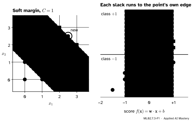
The soft-margin SVM with \({C = 1}\) on the eight points. Right: each point at its score. A point’s slack is how far its score falls short of its own edge, \(+1\) for class \(+1\) and \(-1\) for class \(-1\).
Read the right panel row by row. Points at or beyond their own edge pay nothing. \({(2, 2)}\) is on the correct side but inside the street, and pays \({\xi = 0.5}\). The two new points are on the wrong side and pay more than \(1\) each. The constant \(C\) sets the exchange rate between width and slack.
Build it up
Step 1. Bend the rules. Replace \({y_i f(\vect{x}_i) \ge 1}\) by \({y_i f(\vect{x}_i) \ge 1 - \xi_i}\) with \({\xi_i \ge 0}\). A slack between \(0\) and \(1\) lets a point into the street on its own side; a slack above \(1\) lets it cross the centre line.
Step 2. Pay for the bending. Add \({C \sum_i \xi_i}\) to the objective. A small \(C\) makes slack cheap: the solver buys a wide street and lets many points in. A large \(C\) makes slack dear: the street narrows to keep points out.
Step 3. The best slack is the hinge. For fixed \(\vect{w}\) and \(b\), each \(\xi_i\) only has to satisfy \({\xi_i \ge 0}\) and \({\xi_i \ge 1 - y_i f(\vect{x}_i)}\), and it costs money, so the solver takes the smaller of the two allowed values:
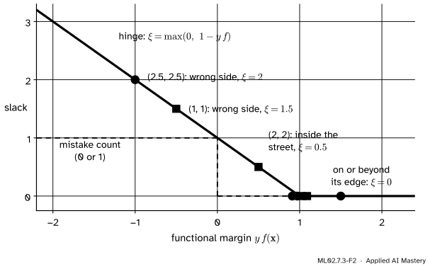
As a function of the functional margin\({y_i f(\vect{x}_i)}\), this is a bent line: zero beyond \(1\), rising with slope \(-1\) below it. It is called the hinge loss.
ML02.7.3-F2
Every point sits on the hinge. The hinge is a convex upper bound on the count of mistakes: it charges a point inside the street even when it is on the correct side.
with \({f(\vect{x}_i) = \vect{w} \cdot \vect{x}_i + b}\).
Stationarity. The derivatives with respect to \(\vect{w}\) and \(b\) are as in lesson 2, giving \({\vect{w} = \sum_i \alpha_i y_i \vect{x}_i}\) and \({\sum_i \alpha_i y_i = 0}\). The new one is
\[
\begin{aligned}
\pd{L}{\xi_i} &= C - \mu_i - \alpha_i = 0 , \\
\text{so}\quad \alpha_i &= C - \mu_i \le C .
\end{aligned}
\]
The dual. Collect the terms of \(L\) that contain \(\xi_i\): \({\xi_i\,(C - \mu_i - \alpha_i)}\), which is zero by the last condition. What remains is exactly the Lagrangian of lesson 2, so the dual objective is unchanged:
where, as in lesson 2, \({S = \sum_{i,j} \alpha_i \alpha_j y_i y_j\, \vect{x}_i \cdot \vect{x}_j}\).
The only change from the hard margin is the ceiling \(C\). A single point can no longer push with unlimited force, which is why one mislabelled point cannot wreck the answer.
Three kinds of point. Complementary slackness now has two parts, \({\alpha_i[y_i f(\vect{x}_i) - 1 + \xi_i] = 0}\) and \({\mu_i \xi_i = 0}\), with \({\mu_i = C - \alpha_i}\):
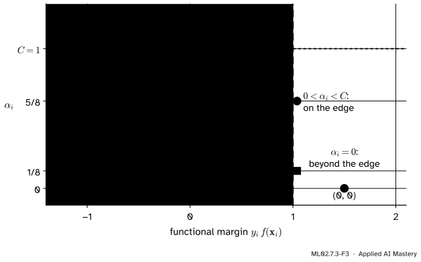
\({\alpha_i = 0}\): then \({\mu_i = C > 0}\), so \({\xi_i = 0}\) and \({y_i f(\vect{x}_i) \ge 1}\). The point is on or beyond its edge and does not affect the answer.
\({0 < \alpha_i < C}\): then \({\mu_i > 0}\), so \({\xi_i = 0}\), and the bracket is zero, so \({y_i f(\vect{x}_i) = 1}\) exactly. The point is on its edge. These points give \(b\).
\({\alpha_i = C}\): then \({\xi_i = 1 - y_i f(\vect{x}_i) \ge 0}\). The point is on its edge, inside the street or on the wrong side.
Points of the last two kinds are the support vectors.
ML02.7.3-F3
The three kinds of point, read from \(\alpha_i\), for the eight points at \({C = 1}\) (the symmetric dual solution). Weights at the ceiling belong to points that pay a slack.
Eliminating the slacks. Put the best slack of Step 3 into the objective:
This is the shape of ridge regression in ML01.9.1: average loss plus \(\lambda\) times the sum of squared weights, with the hinge in place of the squared error. A large \(C\) is a small \(\lambda\): \(C\) is an inverse regularisation strength, like C in LogisticRegression.
Worked example
Eight points, three values of \(C\). The solver (code below) gives:
\(C\)
\(\vect{w}\)
\(b\)
width
\(0.1\)
\({(0.4, 0.4)}\)
\(-1\)
\(3.54\)
\(1\)
\({(0.5, 0.5)}\)
\(-1.5\)
\(2.83\)
\(10\)
\({(0.5, 0.5)}\)
\(-1.5\)
\(2.83\)
ML02.7.3-F4
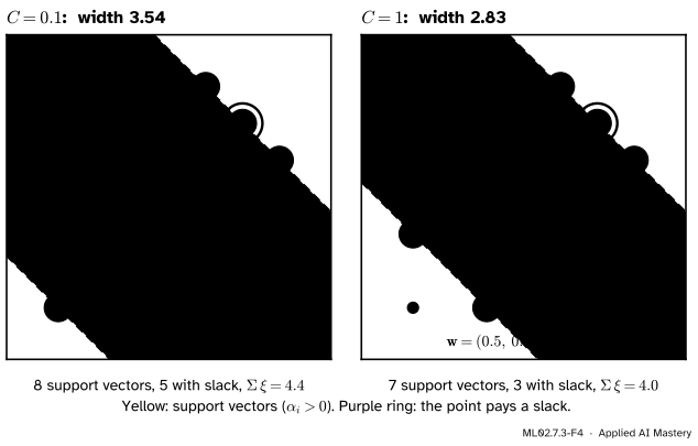
The soft margin for \({C = 0.1}\) and \({C = 1}\). Cheap slack (left) buys a wider street with five points in or across it. Every point is a support vector there.
Check \({C = 1}\) by hand. With \({\vect{w} = (0.5, 0.5)}\) and \({b = -1.5}\) the score is \({0.5\,(x_1 + x_2) - 1.5}\). For \({(2, 2)}\) it is \(0.5\), so \({\xi = 1 - 0.5 = 0.5}\). For \({(1, 1)}\) it is \(-0.5\) and \({y = +1}\), so \({\xi = 1 - (-0.5) = 1.5}\). For \({(2.5, 2.5)}\) it is \(1\) and \({y = -1}\), so \({\xi = 1 + 1 = 2}\). The other five points have \({y f \ge 1}\). The objective is
Check \({C = 0.1}\). The score is \({0.4\,(x_1 + x_2) - 1}\). The slacks are \(0.4\) for \({(1, 0)}\), \({(0, 1)}\) and \({(2, 2)}\), \(1.2\) for \({(1, 1)}\) and \(2\) for \({(2.5, 2.5)}\): a total of \(4.4\), and an objective of \({\tfrac{1}{2}(0.32) + 0.1 \cdot 4.4 = 0.6}\). The dual weights are \(0.08\) for \({(0, 0)}\), \(0.09\) for \({(3, 2)}\) and \({(2, 3)}\), the three points on the edges, and \({C = 0.1}\) for the five that pay.
Why \({C = 10}\) changes nothing. At \({C = 1}\) the dual has many solutions, all with the same \(\vect{w}\) and \(b\). The symmetric one is \({\alpha = 5/8}\) for \({(1, 0)}\) and \({(0, 1)}\), \(1/8\) for \({(3, 2)}\) and \({(2, 3)}\), \(1\) for the three that pay, and \(0\) for \({(0, 0)}\).
Go deeper: the street stops changing at C = 1/4
Keep \({\vect{w} = (0.5, 0.5)}\), \({b = -1.5}\) and try weights \({\alpha = C}\) on the three paying points, \(a\) on \({(1, 0)}\) and \({(0, 1)}\), \(c\) on \({(3, 2)}\) and \({(2, 3)}\), and \(0\) on \({(0, 0)}\). Balance gives \({-2a + C + 2c + C - C = 0}\), so \({a = c + C/2}\). The first coordinate of \({\sum_i \alpha_i y_i \vect{x}_i}\) must be \(0.5\):
Substituting \({a = c + C/2}\) leaves \({4c = 0.5}\), so \({c = 1/8}\) and \({a = C/2 + 1/8}\). The second coordinate gives the same equation, by symmetry. All the conditions of the formal statement hold as long as \({a \le C}\) (a weight at the ceiling with zero slack is allowed), that is \({C \ge 1/4}\). So the same street is optimal for every \({C \ge 1/4}\); a larger \(C\) only raises the weights. For \({C = 10}\), \({a = 5.125}\).
Code
First the reason the hard margin fails: a half-plane is convex, so it cannot hold \({(3, 2)}\) and \({(2, 3)}\) without their midpoint. Then the soft-margin dual, which is lesson 2’s solver with the bounds \({(0, C)}\). \(b\) comes from the points strictly between the bounds.
import numpy as npfrom scipy.optimize import minimizeX = np.array([[0, 0], [1, 0], [0, 1], [2, 2], [3, 2], [2, 3], [1, 1], [2.5, 2.5]], dtype=float)y = np.array([-1, -1, -1, 1, 1, 1, 1, -1], dtype=float)print("midpoint of (3, 2) and (2, 3):", (X[4] + X[5]) /2, " label of that point:", y[7])Q = np.outer(y, y) * (X @ X.T)def soft_svm(C): res = minimize(lambda a: 0.5* a @ Q @ a - a.sum(), np.zeros(len(y)), jac=lambda a: Q @ a -1.0, method="SLSQP", bounds=[(0, C)] *len(y), constraints=[{"type": "eq", "fun": lambda a: a @ y, "jac": lambda a: y}], options={"ftol": 1e-12, "maxiter": 500}) a = res.x w = (a * y) @ X free = (a >1e-6) & (a < C -1e-6) # on the edge: they give b b = np.mean(y[free] - X[free] @ w)return a, w, bdef objective(w, b, C):return0.5* w @ w + C * np.maximum(0, 1- y * (X @ w + b)).sum()for C in (0.1, 1, 10): a, w, b = soft_svm(C) xi = np.maximum(0, 1- y * (X @ w + b))print(f"C = {C:>4}: w = {np.round(w, 3)}, b = {b:.3f}, width {2/ np.linalg.norm(w):.2f}, "f"slacks {np.round(xi, 2)}, objective {objective(w, b, C):.2f}")
midpoint of (3, 2) and (2, 3): [2.5 2.5]  label of that point: -1.0
C =  0.1: w = [0.4 0.4], b = -1.000, width 3.54, slacks [0.  0.4 0.4 0.4 0.  0.  1.2 2. ], objective 0.60
C =    1: w = [0.5 0.5], b = -1.500, width 2.83, slacks [0.  0.  0.  0.5 0.  0.  1.5 2. ], objective 4.25
C =   10: w = [0.5 0.5], b = -1.500, width 2.83, slacks [0.  0.  0.  0.5 0.  0.  1.5 2. ], objective 40.25
The symmetric weights of the worked example are a solution too: they meet every condition and reach the same dual value, whatever weights SLSQP happened to return.
dual =lambda a: a.sum() -0.5* a @ Q @ afor C in (1, 10): sym = np.array([0, C /2+1/8, C /2+1/8, C, 1/8, 1/8, C, C])print(f"C = {C}: symmetric weights {sym}, balance {sym @ y:.1f}, "f"w = {(sym * y) @ X}, dual value {dual(sym):.4f} vs solver {dual(sol[C][0]):.4f}")
C = 1: symmetric weights [0.    0.625 0.625 1.    0.125 0.125 1.    1.   ], balance 0.0, w = [0.5 0.5], dual value 4.2500 vs solver 4.2500
C = 10: symmetric weights [ 0.     5.125  5.125 10.     0.125  0.125 10.    10.   ], balance 0.0, w = [0.5 0.5], dual value 40.2500 vs solver 40.2500
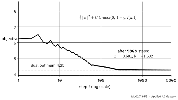
Now the hinge form, minimised directly by subgradient descent (ML01.5). Where \({y_i f(\vect{x}_i) < 1}\) the hinge has slope \({-y_i \vect{x}_i}\) in \(\vect{w}\) and \(-y_i\) in \(b\); elsewhere it is flat. At the corner we take the flat side. The step size shrinks as \({0.05 / \sqrt{t}}\).
def subgradient_svm(C, steps=5000, eta0=0.05): w, b = np.zeros(2), 0.0for t inrange(1, steps +1): inside = y * (X @ w + b) <1# points that pay grad_w = w - C * (y[inside, None] * X[inside]).sum(axis=0) grad_b =-C * y[inside].sum() eta = eta0 / np.sqrt(t) w, b = w - eta * grad_w, b - eta * grad_breturn w, bw_sg, b_sg = subgradient_svm(1.0)print("subgradient descent: w =", np.round(w_sg, 3), " b =", round(b_sg, 3)," objective", round(objective(w_sg, b_sg, 1.0), 4))
subgradient descent: w = [0.501 0.501] b = -1.502 objective 4.2517
ML02.7.3-F6
Subgradient descent on the hinge form reaches the value the dual solver found. The wobbles come from the corner of the hinge: the slope jumps as points cross their edges.
Subgradient descent ends within about \(0.002\) of the dual solution. Last, scikit-learn.
from sklearn.svm import SVCfor C in (0.1, 1, 10): svm = SVC(kernel="linear", C=C, tol=1e-10).fit(X, y)print(f"C = {C:>4}: w = {np.round(svm.coef_[0], 3)}, b = {svm.intercept_[0]:.3f}, "f"{len(svm.support_)} support vectors")
C =  0.1: w = [0.4 0.4], b = -1.000, 8 support vectors
C =    1: w = [0.5 0.5], b = -1.500, 6 support vectors
C =   10: w = [0.5 0.5], b = -1.500, 6 support vectors
scikit-learn agrees on \(\vect{w}\) and \(b\). At \({C = 1}\) and \({C = 10}\) it may list fewer support vectors than the symmetric solution, because it returns another of the equally good weight vectors.
Explore
ML02.7-X1
Margin explorer
Drag the points, or pick one with the buttons and move it with the sliders. Slide \(C\) from \(0.01\) to \(100\) and watch the street, the slacks and the list of weights. Then press Six points and Hard margin for the street of lessons 1 and 2.
Things to try:
At \({C = 1}\), drag \({(1, 1)}\) down towards \({(0, 0)}\). Its slack grows, but its weight is already at the ceiling \({C = 1}\) and the street does not move at all: the weights of the points on the edges shift to make up for it.
Slide \(C\) down to \(0.1\): the street widens to \(3.54\), and the read-out counts eight support vectors.
Slide \(C\) up from \(0.25\) to \(100\): the street does not move, while the weights in the read-out keep growing with \(C\). The “go deeper” note of the worked example explains why.
Pitfalls
ML02.7.3-F5
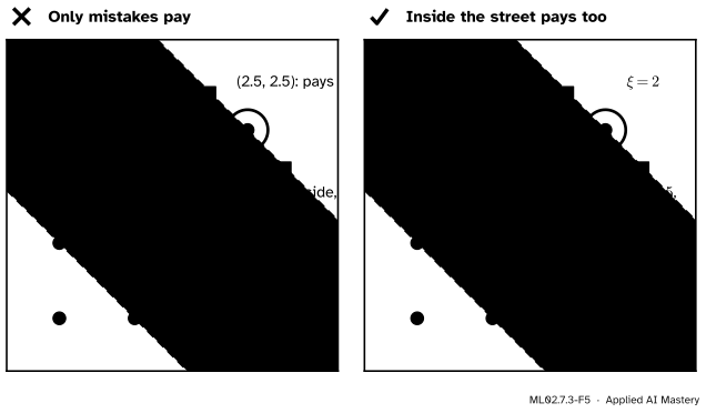
Wrong beside right. \({(2, 2)}\) is classified correctly, yet it pays \({\xi = 0.5}\) because its score is below \(1\).
“The slack counts the training mistakes.”
The slack measures how far a score falls short of its own edge. A point inside the street on the correct side pays a slack below \(1\); a mistake pays more than \(1\). The sum of slacks is an upper bound on the number of training mistakes, not the number itself: here it is \(4\), with \(2\) mistakes.
“A larger C means stronger regularisation, as with a larger lambda.”
It is the other way round: \({\lambda = 1/(2nC)}\). A larger \(C\) fits the training data harder with a narrower street. To add to the confusion, the textbook An Introduction to Statistical Learning uses the letter \(C\) for a budget of total slack, where a larger \(C\) means a wider street. Check which convention a source uses; scikit-learn’s C is the penalty of this lesson.
“The dual weights are unique, like the street.”
The street (\(\vect{w}\) and \(b\)) of the soft margin is unique here, but the weights need not be: at \({C = 1}\) a whole family of weights gives the same street. Compare solvers on \(\vect{w}\), \(b\) and the predictions, not on the list of support vectors.
Check yourself
Recall
1. Write the soft-margin primal problem.
Show answer
Minimise \({\tfrac{1}{2}\norm{\vect{w}}^2 + C\sum_i \xi_i}\) subject to \({y_i(\vect{w} \cdot \vect{x}_i + b) \ge 1 - \xi_i}\) and \({\xi_i \ge 0}\).
2. How does the soft-margin dual differ from the hard-margin dual?
Show answer
Only in the bounds: \({0 \le \alpha_i \le C}\) instead of \({\alpha_i \ge 0}\). The objective and the balance condition are the same.
3. What is the hinge loss of a point with functional margin \({y f(\vect{x}) = 0.3}\)? And with \(1.7\)?
4. Name the three kinds of point by their \(\alpha_i\).
Show answer
\({\alpha_i = 0}\): on or beyond the edge, no influence. \({0 < \alpha_i < C}\): exactly on the edge. \({\alpha_i = C}\): on the edge, inside the street or on the wrong side, paying \({\xi_i = 1 - y_i f(\vect{x}_i)}\).
5. In the form “average hinge loss plus \({\lambda \norm{\vect{w}}^2}\)”, what is \(\lambda\) in terms of \(C\)?
Show answer
\({\lambda = 1/(2nC)}\), so a large \(C\) means weak regularisation.
Exercises
1.★ For \({C = 0.1}\), \({\vect{w} = (0.4, 0.4)}\) and \({b = -1}\), compute the slack of each of the eight points and check the objective \(0.6\).
Show solution
The score is \({0.4\,(x_1 + x_2) - 1}\). Class \(-1\): \({(0, 0)}\) scores \(-1\), slack \(0\); \({(1, 0)}\) and \({(0, 1)}\) score \(-0.6\), slack \({1 - 0.6 = 0.4}\) each; \({(2.5, 2.5)}\) scores \(1\), slack \({1 + 1 = 2}\). Class \(+1\): \({(2, 2)}\) scores \(0.6\), slack \(0.4\); \({(3, 2)}\) and \({(2, 3)}\) score \(1\), slack \(0\); \({(1, 1)}\) scores \(-0.2\), slack \(1.2\). The total slack and the objective are
2.★★ Show that the soft-margin objective with the slacks eliminated, divided by \({nC}\), has the same minimiser as the original, and find \(\lambda\).
Show solution
For any \((\vect{w}, b)\), let \(J(\vect{w}, b)\) be the objective with the slacks eliminated. Dividing by the positive number \({nC}\) gives \({J / (nC)}\), which is smaller at \((\vect{w}_1, b_1)\) than at \((\vect{w}_2, b_2)\) exactly when \(J\) is. So both have the same minimiser. Term by term,
where \(h_i\) is the hinge loss of point \(i\). So \({\lambda = 1/(2nC)}\).
3.★★★ Show that a point with \({y_i f(\vect{x}_i) < 1}\) at the optimum must have \({\alpha_i = C}\), and a point with \({y_i f(\vect{x}_i) > 1}\) must have \({\alpha_i = 0}\).
Show solution
If \({y_i f(\vect{x}_i) < 1}\), the rule \({y_i f(\vect{x}_i) \ge 1 - \xi_i}\) forces \({\xi_i > 0}\). Then \({\mu_i \xi_i = 0}\) gives \({\mu_i = 0}\), and \({\alpha_i = C - \mu_i = C}\).
If \({y_i f(\vect{x}_i) > 1}\), then \({y_i f(\vect{x}_i) - 1 + \xi_i > 0}\) for every \({\xi_i \ge 0}\), so the condition \({\alpha_i[y_i f(\vect{x}_i) - 1 + \xi_i] = 0}\) gives \({\alpha_i = 0}\).
Summary card
Slack lets points into the street, at a price C.
ML02.7.3-F1
Slack is the shortfall to your own edge.
Primal. Minimise \({\tfrac{1}{2}\norm{\vect{w}}^2 + C\sum_i \xi_i}\) with \({y_i f(\vect{x}_i) \ge 1 - \xi_i}\) and \({\xi_i \ge 0}\).
Dual. As before, with \({0 \le \alpha_i \le C}\).
Hinge form. Average hinge \({\max(0, 1 - y_i f(\vect{x}_i))}\) plus \({\lambda \norm{\vect{w}}^2}\), with \({\lambda = 1/(2nC)}\).
Sources. Each was opened and checked against this lesson on 15 November 2026.
Trevor Hastie, Robert Tibshirani and Jerome Friedman, The Elements of Statistical Learning, 2nd edition. Section 12.2.1: the primal (12.8), the Lagrangian (12.9), the conditions (12.10) to (12.12) with \({\alpha_i = C - \mu_i}\), the dual (12.13) with \({0 \le \alpha_i \le C}\), the conditions (12.14) to (12.16), and the remark that points on the edge have \({0 < \alpha_i < C}\) and the rest \({\alpha_i = C}\). Section 12.3.2: the hinge form (12.25) with \({\lambda = 1/C}\) (ESL does not divide the loss by \(n\)).
Gareth James, Daniela Witten, Trevor Hastie and Robert Tibshirani, An Introduction to Statistical Learning, 2nd edition. Section 9.2.2, equations (9.12) to (9.15), uses \(C\) as a budget on the total slack, so a larger \(C\) widens the margin. Section 9.5 rewrites the classifier as hinge loss plus a ridge penalty (9.25) and notes that only support vectors affect it.
Kilian Weinberger, Lecture 9: SVM, Cornell CS4780, Fall 2018: slack variables, the optimal slack \({\max(1 - y_i(\vect{w}\T\vect{x}_i + b), 0)}\), the unconstrained hinge form, and large and small \(C\).
scikit-learn 1.9 User Guide, Section 1.4.7.1: the SVC primal with slacks and penalty \(C\), the dual with \({0 \le \alpha_i \le C}\), and the equivalent hinge-loss form.
Next.ML02.7.4 Linear SVMs in practice takes the soft margin to a real dataset, with scaling, a cross-validated \(C\) and a regression version.