A linear SVM on real data: why the features must be scaled first and inside a pipeline, how to choose C by cross-validation, how the SVM compares with logistic regression, and how support vector regression fits a tube instead of a line.
ML02.7.4L2 Intermediate25 minIn review (what this means)
The maths and code on this page are checked by automated tests on every change, but an independent reader has not signed it off yet. Spot a mistake or a confusing step? Tell us.
Explain why an SVM is not scale invariant and fit it inside a pipeline with StandardScaler.
Choose C by cross-validation with GridSearchCV and report an honest test accuracy.
Compare the hinge loss with the log loss and say when an SVM and logistic regression differ, including the lack of probabilities.
Describe support vector regression by its epsilon-insensitive tube and fit SVR on a small data set by hand and in code.
The question
The breast cancer dataset that ships with scikit-learn describes 569 tumours by 30 measurements, from a “worst area” of about \(880\) on average to a “fractal dimension error” of about \(0.004\). Fit a linear SVM to it. What must you do to the features first, how do you choose \(C\), and is the result any different from logistic regression?
From the last lesson
1. What is the hinge loss of a point, and when is it zero?
Show answer
\({\max(0,\ 1 - y_i f(\vect{x}_i))}\). It is zero when \({y_i f(\vect{x}_i) \ge 1}\): the point is on or beyond its own edge of the street.
2. Does a larger \(C\) mean stronger or weaker regularisation?
Show answer
Weaker. In the form “average hinge loss plus \({\lambda \norm{\vect{w}}^2}\)”, \({\lambda = 1/(2nC)}\).
Intuition
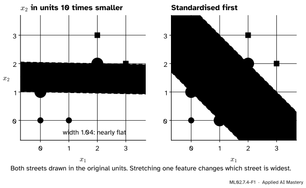
The SVM maximises a distance, and a distance adds up squared differences in every feature. A feature recorded in large units dominates that sum; one recorded in tiny units hardly counts. So the widest street depends on the units, which have nothing to do with the classes.
ML02.7.4-F1
The same six points. Record \(x_2\) in units ten times smaller and the SVM, measuring distance in those units, finds a nearly flat street, half as wide in the original units. Standardising first restores the street of lesson 1.
The cure is to put every feature on the same footing before the SVM sees it. Standardising subtracts each feature’s mean and divides by its standard deviation, so that every feature has mean \(0\) and spread \(1\). For the six points the two features already have the same spread, so standardising leaves the street of lesson 1 as it was.
Build it up
Step 1. Scale inside a pipeline. The means and standard deviations are themselves learned from data, so they must come from the training rows only. A Pipeline of StandardScaler and SVC fits both steps on whatever rows it is given, which keeps every validation fold and the test set out of the scaling.
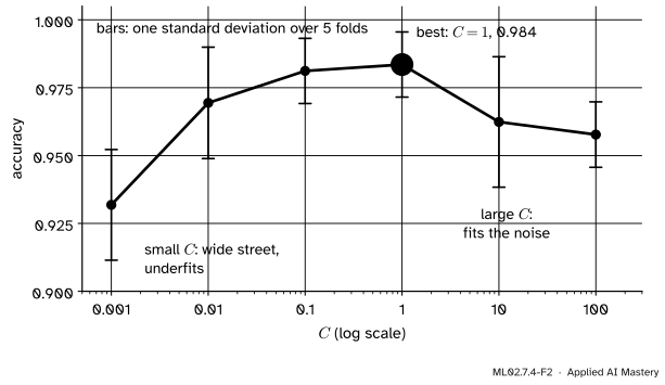
Step 2. Choose \(C\) on validation folds.\(C\) trades width for slack, and the training data cannot judge it: a larger \(C\) always fits the training rows at least as hard. So try a grid of values, \(0.001\) to \(100\) in factors of ten, and score each by 5-fold cross-validation (ML01.9.3).
ML02.7.4-F2
Cross-validated accuracy of a standardised linear SVM against \(C\). The peak is at \({C = 1}\); the bars show how much the five folds disagree, which is as large as most of the differences.
Step 3. Test once. Refit the chosen model on all the training rows and score it once on the test rows, which played no part in any choice.
Step 4. Read the support vectors. The fitted SVM keeps only the rows with \({\alpha_i > 0}\). On this data it keeps 29 of 426.
The formal statement
Hinge against log loss. Both the soft-margin SVM and logistic regression fit a linear score \({f(\vect{x}) = \vect{w} \cdot \vect{x} + b}\) by minimising a loss of the margin \({m = y f(\vect{x})}\) plus a ridge penalty, with labels \({y \in \{-1, +1\}}\):
The second is the log loss of ML01.6.2 rewritten for labels \(\pm 1\): with \({p = \sigma(f)}\), a point of class \(+1\) costs \({-\ln \sigma(f) = \ln(1 + e^{-f})}\) and a point of class \(-1\) costs \({-\ln(1 - \sigma(f)) = \ln(1 + e^{f})}\), and both are \({\ln(1 + e^{-y f})}\).
ML02.7.4-F3
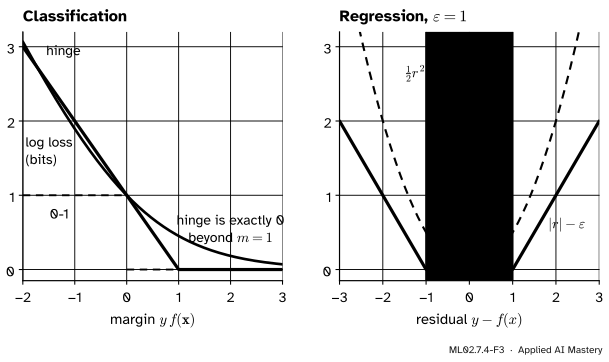
The losses side by side, with the log loss drawn in bits (divided by \({\ln 2}\)) so that it also passes through \(1\) at \({m = 0}\). The hinge is exactly zero beyond \({m = 1}\); the log loss never is. In regression the \(\varepsilon\)-insensitive loss ignores residuals smaller than \(\varepsilon\).
Far on the wrong side both losses grow like \({-m}\), so they agree about bad mistakes. They differ beyond \({m = 1}\): the hinge is exactly zero there, so those points drop out of the fit, while the log loss still pulls on every point a little. Hence:
the SVM depends only on its support vectors (ISL Section 9.5), logistic regression on all rows;
logistic regression estimates a probability \({\sigma(f)}\); the SVM score \(f\) is not a probability. scikit-learn’s SVC offers probability=True, which fits a logistic curve to the scores with an extra internal cross-validation (Platt scaling, ML04.7).
Support vector regression. For a numeric target, replace the street by a tube of half-height \(\varepsilon\) around \({f(x) = \vect{w} \cdot \vect{x} + b}\). Residuals inside the tube cost nothing; outside, the cost grows linearly:
The \({\tfrac{1}{2}\norm{\vect{w}}^2}\) term asks for the flattest function, as the margin asked for the shortest \(\vect{w}\). Points inside the tube get dual weight \(0\); only points on or outside its edges are support vectors.
Worked example
SVR on the eight-point set. The data are \({x = 1, \dots, 8}\) with \({y = (1, 2, 2, 4, 6, 7, 7, 9)}\). Take \({\varepsilon = 1}\) and ask first for the flattest line whose tube holds every point.
ML02.7.4-F4
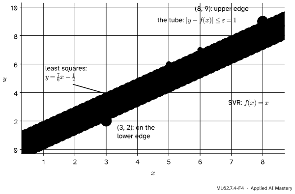
The flattest line whose tube of half-height \(1\) holds all eight points. It is pinned by \({(3, 2)}\) on the lower edge and \({(8, 9)}\) on the upper edge.
Which points pin it? A line \({f(x) = wx + b}\) keeps \({(3, 2)}\) in the tube only if \({2 - (3w + b) \ge -1}\), and \({(8, 9)}\) only if \({9 - (8w + b) \le 1}\). Rearranged:
\[
\begin{aligned}
b &\le 3 - 3w, \\
b &\ge 8 - 8w .
\end{aligned}
\]
Both hold only if \({8 - 8w \le 3 - 3w}\), that is \({5 \le 5w}\), so \({w \ge 1}\). The flattest choice is \({w = 1}\), and then \({0 \le b \le 0}\) forces \({b = 0}\).
Check the rest. With \({f(x) = x}\) the residuals are \({(0, 0, -1, 0, 1, 1, 0, 1)}\): none exceeds \(1\) in size, so every point is in the tube and the loss term is \(0\). Besides \({(8, 9)}\), the points \({(5, 6)}\) and \({(6, 7)}\) also touch the upper edge. The least-squares line, \({y = \tfrac{7}{6}x - \tfrac{1}{2}}\), is steeper: it listens to every residual, while SVR ignores residuals up to \(1\).
With the penalty. For a finite \(C\) the solver may prefer a flatter line that lets some points out of the tube. Lowering \(w\) from \(1\) to \({1 - \delta}\) saves less than \(\delta\) in \({\tfrac{1}{2}w^2}\). But \({(3, 2)}\) then sticks out below the tube by at least \({3w + b - 3}\) and \({(8, 9)}\) above it by at least \({8 - 8w - b}\). These add up to \({5 - 5w = 5\delta}\), whatever \(b\) is, at a cost of at least \({5C\delta}\). For \({C = 1}\) that is a bad trade, so \({f(x) = x}\) is also the answer of SVR with \({C = 1}\).
Code
First the data and the case for scaling: the spreads of the 30 features.
import numpy as npfrom sklearn.datasets import load_breast_cancerdata = load_breast_cancer()X, y = data.data, data.target # y = 1 for benign, 0 for malignantspread = X.std(axis=0)print(X.shape, " class counts:", np.bincount(y))print(f"largest spread: {data.feature_names[spread.argmax()]}, {spread.max():.1f}")print(f"smallest spread: {data.feature_names[spread.argmin()]}, {spread.min():.4f}")print(f"ratio: {spread.max() / spread.min():,.0f}")
(569, 30)   class counts: [212 357]
largest spread: worst area, 568.9
smallest spread: fractal dimension error, 0.0026
ratio: 215,171
The six points of the anchor figure, from scratch: multiply \(x_2\) by 10, fit the hard margin, and read the street back in the original units. Then standardise by hand.
from sklearn.svm import SVCP = np.array([[0, 0], [1, 0], [0, 1], [2, 2], [3, 2], [2, 3]], dtype=float)labels = np.array([-1, -1, -1, 1, 1, 1])stretched = P * [1, 10]svm = SVC(kernel="linear", C=1e6, tol=1e-10).fit(stretched, labels)w_orig = svm.coef_[0] * [1, 10] # the same score, in the original unitsprint("support vectors:", P[svm.support_].tolist())print("width in original units:", round(2/ np.linalg.norm(w_orig), 2))Z = (stretched - stretched.mean(axis=0)) / stretched.std(axis=0)svm_z = SVC(kernel="linear", C=1e6, tol=1e-10).fit(Z, labels)print("after standardising, support vectors:", P[svm_z.support_].tolist())
support vectors: [[0.0, 1.0], [2.0, 2.0]]
width in original units: 1.04
after standardising, support vectors: [[1.0, 0.0], [0.0, 1.0], [2.0, 2.0]]
Now the real data: a stratified split, then \(C\) by 5-fold cross-validation with the scaler inside the pipeline, and one test.
mean CV accuracy: [0.932 0.969 0.981 0.984 0.962 0.958]
best C: 1.0
test: 138 of 143 correct; support vectors kept: 29 of 426
The SVM keeps 29 rows. Refit it on those rows alone and nothing changes; do the same to logistic regression and its weights move.
from sklearn.linear_model import LogisticRegressionscaler = StandardScaler().fit(X_train)Z_train = scaler.transform(X_train)full = SVC(kernel="linear", C=1.0, tol=1e-8).fit(Z_train, y_train)keep = full.support_again = SVC(kernel="linear", C=1.0, tol=1e-8).fit(Z_train[keep], y_train[keep])print("SVM, largest change in a weight:", f"{np.abs(full.coef_ - again.coef_).max():.1e}")logistic = LogisticRegression(C=1.0).fit(Z_train, y_train)logistic_kept = LogisticRegression(C=1.0).fit(Z_train[keep], y_train[keep])print("logistic, largest change in a weight:", round(float(np.abs(logistic.coef_ - logistic_kept.coef_).max()), 2))pred_svm = model.predict(X_test)pred_lr = make_pipeline(StandardScaler(), LogisticRegression(C=1.0)).fit(X_train, y_train).predict(X_test)print("test predictions that agree:", int((pred_svm == pred_lr).sum()), "of", len(y_test))print("SVC has predict_proba:", hasattr(model, "predict_proba"))
SVM, largest change in a weight: 2.6e-08
logistic, largest change in a weight: 0.87
test predictions that agree: 140 of 143
SVC has predict_proba: False
LinearSVC solves the linear problem with a different library and is much faster on large data, but by default it minimises the squared hinge and also penalises the bias, so its answers differ a little.
from sklearn.svm import LinearSVCfor loss in ("squared_hinge", "hinge"): fast = make_pipeline(StandardScaler(), LinearSVC(C=1.0, loss=loss, max_iter=100_000)).fit(X_train, y_train)print(f"LinearSVC, loss={loss}: {int((fast.predict(X_test) == y_test).sum())} of {len(y_test)} correct")
LinearSVC, loss=squared_hinge: 136 of 143 correct
LinearSVC, loss=hinge: 138 of 143 correct
Last, support vector regression on the eight points: the hard tube from scratch with SLSQP, then SVR.
from scratch: w = 1.0  b = -0.0
SVR: w = [1.]  b = [0.]
residuals: [ 0.  0. -1.  0.  1.  1.  0.  1.]
least squares: [ 1.1667 -0.5   ]
Explore
The margin explorer is in lesson 3. Press Six points and Hard margin, then select \({(0, 1)}\) and drag it upwards slowly. The street turns to keep it out: one support vector is enough to tilt the answer, which is why a feature with a large spread, which moves points far, can tilt the street too.
Pitfalls
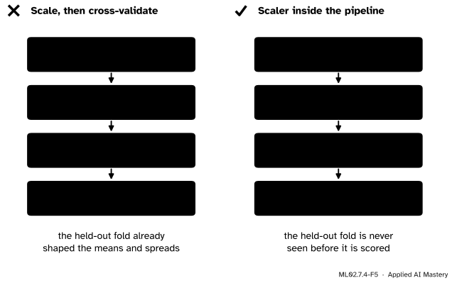
ML02.7.4-F5
Wrong beside right. Fitted once on all rows, the scaler has already seen every validation fold. Inside the pipeline it is refitted on the training part of each fold.
“Scaling is a preprocessing step, so do it once at the start.”
The scaler learns means and spreads, and that learning must not see validation or test rows. Put StandardScaler and the SVM in one pipeline and hand the pipeline to GridSearchCV. The leak is small for a scaler but large for steps that learn more, such as feature selection (ML04.3).
“The SVM score is a probability, or close to one.”
decision_function returns \({\vect{w} \cdot \vect{x} + b}\), a signed distance in units of \({1/\norm{\vect{w}}}\), not a probability, and SVC has no predict_proba unless it is built with probability=True. That option fits a logistic curve to the scores by internal cross-validation; the scikit-learn guide warns that it is expensive and that the probabilities can be inconsistent with the scores.
“LinearSVC and SVC(kernel=‘linear’) are the same model.”
They solve slightly different problems: LinearSVC uses the squared hinge by default and penalises the bias along with the weights. On this split it gets 136 test rows right against 138 for SVC; with loss="hinge" it matches 138. Use LinearSVC for large data, and state the loss.
Check yourself
Recall
1. Why must the features be scaled before a linear SVM?
Show answer
The SVM maximises a Euclidean distance, which is dominated by features with large spreads, so the widest street depends on the units. Standardising gives every feature mean \(0\) and spread \(1\).
2. Why should the scaler sit inside the pipeline?
Show answer
Its means and spreads are learned from data. Inside the pipeline they are learned from the training part of each fold only, so no validation or test row leaks into the model.
3. Name two differences between a linear SVM and logistic regression.
Show answer
The SVM depends only on its support vectors, because the hinge is exactly zero beyond margin \(1\); logistic regression depends on every row. Logistic regression gives probabilities; the SVM gives a score that is not a probability.
4. What does the \(\varepsilon\)-insensitive loss charge for a residual of \(0.6\) and of \(2.5\) when \({\varepsilon = 1}\)?
5. Which \(C\) did cross-validation choose on the breast cancer data, and how many support vectors did the model keep?
Show answer
\({C = 1}\), with a mean CV accuracy of \(0.984\), and 29 support vectors out of 426 training rows.
Exercises
1.★ A standardised linear SVM gives a tumour the score \({f = -0.4}\). Which class is predicted, and is the tumour inside the street?
Show solution
The score is negative, so the class with label \(-1\), here class \(0\) (malignant) in scikit-learn’s coding. Since \({\abs{f} = 0.4 < 1}\), the point lies inside the street: the model is not confident, and a training point there would pay a slack of \({1 - 0.4 = 0.6}\).
2.★★ With \({\varepsilon = 1.5}\), find the flattest line whose tube holds the eight points. Which points pin it?
Show solution
Try the same pair. \({(3, 2)}\) stays in the tube if \({2 - 3w - b \ge -1.5}\), that is \({b \le 3.5 - 3w}\); \({(8, 9)}\) if \({9 - 8w - b \le 1.5}\), that is \({b \ge 7.5 - 8w}\). Both hold when \({7.5 - 8w \le 3.5 - 3w}\), so \({w \ge 0.8}\). With \({w = 0.8}\), \({b = 3.5 - 2.4 = 1.1}\). Check all points: the residuals of \({f(x) = 0.8x + 1.1}\) for \({x = 1, \dots, 8}\) are
all within \(1.5\) in size. So \({f(x) = 0.8x + 1.1}\), pinned by \({(3, 2)}\) below and \({(8, 9)}\) above. A wider tube allows a flatter line.
3.★★★ Show that for labels \(\pm 1\) the log loss of logistic regression is \({\ln(1 + e^{-y f})}\), and that both it and the hinge grow like \({-y f}\) when \({y f}\) is very negative.
Show solution
With \({p = \sigma(f) = 1/(1 + e^{-f})}\), a class \(+1\) point costs \({-\ln p = \ln(1 + e^{-f})}\). A class \(-1\) point costs \({-\ln(1 - p)}\), and \({1 - \sigma(f) = \sigma(-f)}\), so the cost is \({\ln(1 + e^{f})}\). Both are \({\ln(1 + e^{-yf})}\) with \({y = \pm 1}\).
Write \({m = yf}\). For very negative \(m\), \({e^{-m}}\) is huge, so \({\ln(1 + e^{-m}) = -m + \ln(1 + e^{m})}\) and \({\ln(1 + e^{m}) \to 0}\): the log loss behaves like \(-m\). The hinge is \({1 - m}\) there, which also grows like \(-m\). Both charge bad mistakes linearly, unlike the squared loss.
Summary card
Scale inside a pipeline, choose C on folds, test once.
Choose \(C\). Grid from \(0.001\) to \(100\), 5-fold CV: \({C = 1}\), accuracy \(0.984\), then 138 of 143 on test.
Hinge vs log. Same behaviour on mistakes; the hinge is zero beyond margin \(1\), so only support vectors matter, and no probabilities.
SVR. Flattest \(f\) with \({\abs{y - f} \le \varepsilon}\) where possible; eight points, \({\varepsilon = 1}\): \({f(x) = x}\).
Sources and next steps
Sources. Each was opened and checked against this lesson on 15 November 2026.
scikit-learn 1.9 User Guide, Section 1.4 Support Vector Machines. Section 1.4.5: “Support Vector Machine algorithms are not scale invariant, so it is highly recommended to scale your data”, with a make_pipeline(StandardScaler(), SVC()) example. Section 1.4.1: LinearSVC uses the squared hinge loss and also regularises the intercept. Section 1.4.1.2: probability=True calibrates scores with Platt scaling, fitted by an extra cross-validation, and the probabilities may be inconsistent with the scores. Section 1.4.7.2: the SVR primal, which penalises samples whose prediction is at least \(\varepsilon\) from the target.
Gareth James, Daniela Witten, Trevor Hastie and Robert Tibshirani, An Introduction to Statistical Learning, 2nd edition, Section 9.5: the hinge loss against the logistic loss, only support vectors affecting the classifier, and the two methods often giving very similar results.
Trevor Hastie, Robert Tibshirani and Jerome Friedman, The Elements of Statistical Learning, 2nd edition, Section 12.3.2: the SVM as loss plus penalty, equation (12.25), compared with other losses in Figure 12.4.
Next. Module ML02.8, The kernel trick, replaces the dot products of the dual with kernels and gives the SVM curved boundaries. Calibrating SVM scores into probabilities is in ML04.7.