AdaBoostClassifier with stumps on the breast cancer data: the number of rounds, the learning rate as shrinkage, test error that keeps falling after training error reaches zero, what flipped labels do to the weights, and a fair comparison with a random forest.
ML02.3.4L2 Intermediate25 minIn review (what this means)
The maths and code on this page are checked by automated tests on every change, but an independent reader has not signed it off yet. Spot a mistake or a confusing step? Tell us.
Fit AdaBoostClassifier with stumps, read its staged errors, and choose n_estimators and learning_rate.
Explain the learning rate as shrinkage of every alpha_m and its trade-off with the number of rounds.
Show with numbers how flipped labels draw AdaBoost’s weight and hurt its test error.
Compare AdaBoost with a random forest of the same size on the same splits, and name SAMME and AdaBoostRegressor.
The question
On twelve points we could follow every weight. On the 569 tumours of load_breast_cancer, each with 30 measurements, we cannot. How many stumps should AdaBoost use, what does its learning_rate do, and what happens when some of the training labels are simply wrong, as they are in any real data set?
From the last lesson
1. With the exponential loss, what are AdaBoost’s weights?
Show answer
\({w_i^{(m)} = e^{-y_i F_{m-1}(x_i)}}\): the current exponential loss of each point.
2. State the training-error bound.
Show answer
Training error \(\le \prod_m 2\sqrt{\epsilon_m(1-\epsilon_m)} \le \exp(-2\sum_m \gamma_m^2)\), with \({\gamma_m = \tfrac12 - \epsilon_m}\).
Intuition
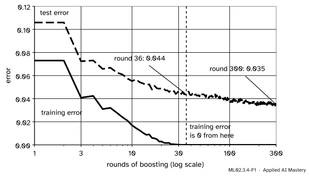
Run AdaBoost with stumps and watch two curves: the error on the training data and the error on held-out test data. The training error falls to zero within a few dozen rounds, as lesson ML02.3.3 promised. The surprise is the test error.
ML02.3.4-F1
Averaged over 20 splits, the training error is zero from round 36 on, yet the test error keeps falling, from \(0.044\) at round 36 to \(0.035\) at round 300.
Once every training point is right, why should more stumps help? Lesson ML02.3.3 gave the clue: the exponential loss keeps falling after the training error is zero, because the margins keep growing. A vote that is right by a wide margin on every training point tends to generalise better than one that is barely right. That is the margin explanation of Schapire and colleagues, which ML06.9 treats properly. It is a tendency, not a law, as the noisy data later in this lesson shows.
Build it up
Step 1. The library call.AdaBoostClassifier takes a weak learner (by default a DecisionTreeClassifier with max_depth=1), a number of rounds n_estimators (default 50) and a learning_rate (default 1). After fitting, staged_predict gives the prediction after each round, which is how the curves above were drawn.
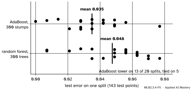
Step 2. A fair opponent. A random forest (ML02.2.3) is the natural comparison: also an ensemble of trees, but deep trees built independently. On the same splits, with 300 members each, AdaBoost’s stumps did better on average.
ML02.3.4-F5
AdaBoost against a random forest of the same size, each dot one split of 143 test points. The means differ by about one tumour in a hundred, and the spread within each row is much wider than that gap.
The spread matters as much as the means: on any one split either model can win, and ML02.11.3 shows how to compare models fairly with repeated folds.
Step 3. More than two classes, and regression. With \(K\) classes, scikit-learn runs SAMME, which adds \({\ln(K-1)}\) to each learner weight; for \({K = 2}\) that term is \({\ln 1 = 0}\) and SAMME is the algorithm of this module (with the doubled \(\alpha\) of ML02.3.2). Lesson ML02.10.2 explains where the extra term comes from. For regression there is AdaBoostRegressor, which runs a variant called AdaBoost.R2; gradient boosting (ML02.4) is the more common choice for numbers.
The formal statement
The learning rate is shrinkage. With learning rate \(\nu\), scikit-learn uses the learner weight
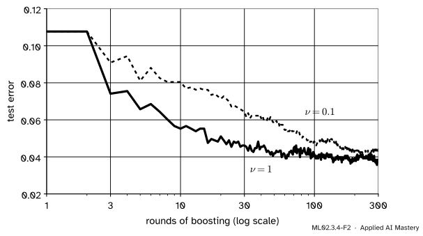
and multiplies the weight of each miss by \(e^{a_m}\) before rescaling. For two classes this is the algorithm of ML02.3.2 with every step \(\alpha_m\) multiplied by \(\nu\). With \({\nu = 1}\) the newest learner’s misses end at exactly half the weight; with \({\nu < 1}\) they end below half, so each round moves the weights less, and more rounds are needed to go as far.
ML02.3.4-F2
A smaller learning rate takes smaller steps. On clean data it needs many more rounds to reach the same test error; the payoff comes with noisy labels, below.
How much less than half. With \({\nu < 1}\) and the update written as in ML02.3.2, the misses end with the share
which is \(\tfrac12\) at \({\nu = 1}\) and smaller for \({\nu < 1}\). For the first stump of the twelve points, with \({\epsilon = \tfrac16}\) and \({e^{\alpha} = \sqrt5}\), and with \({\nu = \tfrac12}\), the factor is \(5^{1/4}\), and the share simplifies to
Weights grow exponentially in the margin. Lesson ML02.3.3 showed that after \(m\) rounds the weight of point \(i\) is proportional to \({e^{-y_i F_m(x_i)}}\). Two points whose margins differ by \(\Delta\) have weights in the ratio \(e^{\Delta}\). A training point whose label is wrong is one the weak learners keep disagreeing with, so its margin is driven negative and its weight grows round after round, until a few such points carry a large share of all the weight.
Worked example
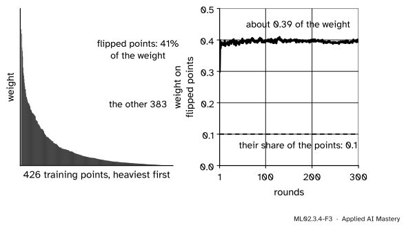
Flip 10 percent of the labels. Split load_breast_cancer into 426 training and 143 test tumours, stratified, with random_state=0. Flip the label of 43 training points, about 10 percent, chosen with a seeded generator, and fit AdaBoost with 300 stumps. Then track the share of the total weight held by the 43 flipped points:
after round 1: \(0.30\), three times their share of the points;
after round 100: \(0.41\);
after round 300: \(0.41\).
Of the 43 heaviest training points at the end, 34 are flipped ones. The run drives the training error on the noisy labels down to about \(0.012\), so it has fitted almost all of the wrong labels, and its test error, measured against the true labels, is \(0.077\), against \(0.056\) for the same run on clean labels.
ML02.3.4-F3
With 10 percent of the labels flipped, the flipped points end up holding about 40 percent of the weight. Every later stump is chosen mainly to please them.
Code
Clean labels first: five stratified splits, with the staged errors averaged, and a random forest of the same size on the same splits.
import numpy as npfrom sklearn.datasets import load_breast_cancerfrom sklearn.ensemble import AdaBoostClassifier, RandomForestClassifierfrom sklearn.model_selection import StratifiedShuffleSplit, train_test_splitfrom sklearn.tree import DecisionTreeClassifierX, y = load_breast_cancer(return_X_y=True)stump = DecisionTreeClassifier(max_depth=1)splits = StratifiedShuffleSplit(n_splits=5, test_size=0.25, random_state=0).split(X, y)train_err, test_err, forest_err = [], [], []for a, b in splits: ada = AdaBoostClassifier(stump, n_estimators=300, random_state=0).fit(X[a], y[a]) train_err.append([np.mean(p != y[a]) for p in ada.staged_predict(X[a])]) test_err.append([np.mean(p != y[b]) for p in ada.staged_predict(X[b])]) rf = RandomForestClassifier(n_estimators=300, random_state=0).fit(X[a], y[a]) forest_err.append(np.mean(rf.predict(X[b]) != y[b]))train_err, test_err = np.mean(train_err, axis=0), np.mean(test_err, axis=0)first_zero =int(np.argmax(train_err ==0)) +1print("training error is 0 from round", first_zero)print("test error at rounds 10, 30, 100, 300:", np.round(test_err[[9, 29, 99, 299]], 3))print("random forest, 300 trees:", round(np.mean(forest_err), 3))
training error is 0 from round 29
test error at rounds 10, 30, 100, 300: [0.056 0.055 0.053 0.043]
random forest, 300 trees: 0.052
The training error reached zero near round 29, while the test error went on falling, to about \(0.043\) at round 300; the forest averaged about \(0.052\).
The learning rate scales every learner weight. Then the noisy run: the weight of each point after \(m\) rounds is proportional to \(\exp\big(\sum_{k \le m} a_k\, I[\text{stump } k \text{ misses it}]\big)\).
X_tr, X_te, y_tr, y_te = train_test_split(X, y, test_size=0.25, stratify=y, random_state=0)half = AdaBoostClassifier(stump, n_estimators=1, learning_rate=0.5, random_state=0).fit(X_tr, y_tr)full = AdaBoostClassifier(stump, n_estimators=1, learning_rate=1.0, random_state=0).fit(X_tr, y_tr)print("first learner weight, nu = 0.5 and nu = 1:", half.estimator_weights_, full.estimator_weights_)flip = np.random.default_rng(0).choice(len(y_tr), size=43, replace=False)noisy = y_tr.copy()noisy[flip] =1- noisy[flip]def run(labels): ada = AdaBoostClassifier(stump, n_estimators=300, random_state=0).fit(X_tr, labels) missed = np.array([s.predict(X_tr) != labels for s in ada.estimators_]) log_w = np.cumsum(ada.estimator_weights_[:, None] * missed, axis=0) w = np.exp(log_w - log_w.max(axis=1, keepdims=True))return ada, w / w.sum(axis=1, keepdims=True)clean_model, _ = run(y_tr)noisy_model, w = run(noisy)share = w[:, flip].sum(axis=1)print("weight share of the flipped points after rounds 1, 100, 300:", np.round(share[[0, 99, 299]], 2))print("flipped among the 43 heaviest:", np.isin(np.argsort(-w[-1])[:43], flip).sum())print("training error on noisy labels:", round(np.mean(noisy_model.predict(X_tr) != noisy), 3))print("test error, clean and noisy training:",round(np.mean(clean_model.predict(X_te) != y_te), 3), round(np.mean(noisy_model.predict(X_te) != y_te), 3))
first learner weight, nu = 0.5 and nu = 1: [1.29010841] [2.58021683]
weight share of the flipped points after rounds 1, 100, 300: [0.3  0.41 0.41]
flipped among the 43 heaviest: 34
training error on noisy labels: 0.012
test error, clean and noisy training: 0.056 0.077
These runs depend on a seeded split and seeded flips; on another machine the last digit of an error can differ, which is why the checks above allow a small tolerance.
Explore
The AdaBoost stepper in ML02.3.2 shows the same pile-up on a small scale. With stumps, the points \((2,5)\) and \((5,5)\), which no stump can fit together with their neighbours, take half of all the weight in round 1 and keep between about two fifths and one half of it from then on, while the other two corners of the pattern of ML02.3.3, \((2,3)\) and \((5,3)\), slowly gain weight too: the hard points end up with most of it, just as the flipped tumours do here.
Pitfalls
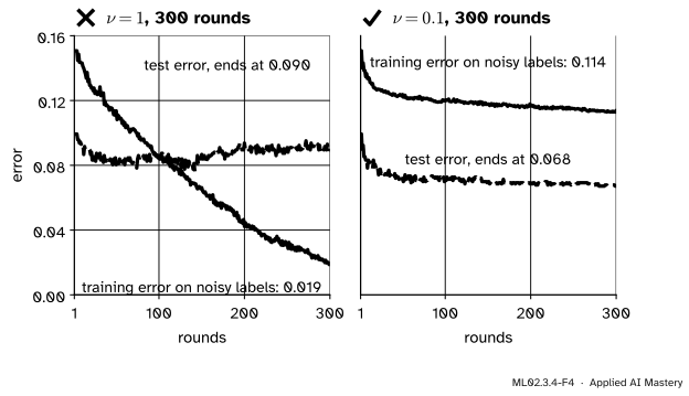
ML02.3.4-F4
Wrong beside right, with 10 percent of the labels flipped. Full-size steps chase the flipped labels until the training error is nearly zero and the test error rises. Small steps fit them far less and end with a lower test error.
“More rounds always help AdaBoost.”
On clean data they often do, because the margins keep growing. With wrong labels, every extra round fits the noise a little more: in the figure the training error on the noisy labels falls to \(0.019\) while the test error climbs back to \(0.090\). Choose the number of rounds on validation data, with staged_predict, and prefer a smaller learning rate when labels are unreliable.
“Training error is zero, so the model is finished.”
AdaBoost does not stop when the training error reaches zero, and on clean data the test error kept falling for hundreds of rounds after it. The stopping point is a validation question, not a training one. (scikit-learn stops early only if a learner fits the weighted training data perfectly, or if its weighted error is no better than a coin’s.)
“The learning rate only changes the speed, not the answer.”
With a fixed number of rounds it changes the answer: a small \(\nu\) with 300 rounds is a different model from \({\nu = 1}\) with 300 rounds. The two settings trade off, and they must be tuned together.
Check yourself
Recall
1. What weak learner does AdaBoostClassifier use by default?
Show answer
A decision stump: DecisionTreeClassifier with max_depth=1.
2. What does learning_rate do to each learner weight?
Show answer
It multiplies it: the learner weight becomes \(\nu\) times \({\ln\big((1-\epsilon_m)/\epsilon_m\big) + \ln(K-1)}\).
3. On clean load_breast_cancer splits, what did the test error do after the training error reached zero?
Show answer
It kept falling, from about \(0.055\) near round 30 to about \(0.043\) at round 300 in the lesson’s five splits.
4. With 10 percent of the training labels flipped, what share of the weight did the flipped points hold after 300 rounds?
Show answer
About \(0.41\), four times their share of the points.
5. What term does SAMME add to the learner weight, and why does it vanish for two classes?
Show answer
\({\ln(K-1)}\), which is \({\ln 1 = 0}\) when \({K = 2}\).
Exercises
1.★ A two-class run uses \({\nu = 0.5}\), and a round’s stump has weighted error \(0.2\). What learner weight does scikit-learn store, and by what factor are the stump’s misses multiplied before rescaling?
Show solution
\(a = 0.5 \left(\ln \tfrac{0.8}{0.2} + \ln 1\right) = 0.5 \ln 4 = \ln 2 \approx 0.693\). The misses are multiplied by \({e^{a} = 2}\) and the correct points are left alone before the rescaling.
2.★★ After some rounds, one training point has margin \({-2}\) and another has margin \({+2}\). How many times heavier is the first?
Show solution
Weights are proportional to \({e^{-yF}}\), so the ratio is \({e^{2}/e^{-2} = e^{4} \approx 54.6}\). One badly misclassified point weighs as much as about 55 well-classified ones, and the next stump is fitted with that in mind.
3.★★★ Show that with \({\nu < 1}\) the newest learner’s misses hold less than half the weight after the update, and check the value \({1/(1+\sqrt5)}\) for \({\epsilon = \tfrac16}\) and \({\nu = \tfrac12}\).
Show solution
The share is
\[
s = \frac{\epsilon e^{\nu\alpha}}{\epsilon e^{\nu\alpha} + (1-\epsilon)e^{-\nu\alpha}} ,
\]
and \({s < \tfrac12}\) exactly when \({\epsilon e^{\nu\alpha} < (1-\epsilon) e^{-\nu\alpha}}\), that is when \({e^{2\nu\alpha} < (1-\epsilon)/\epsilon = e^{2\alpha}}\). For \({\epsilon < \tfrac12}\) we have \({\alpha > 0}\), so this holds for every \({\nu < 1}\). With \({\epsilon = \tfrac16}\), \({e^{\alpha} = \sqrt5}\) and \({\nu = \tfrac12}\), the factor is \({e^{\nu\alpha} = 5^{1/4}}\). Multiply the top and bottom of \(s\) by \(6 \cdot 5^{1/4}\):
Noise. Weights grow like \({e^{-yF}}\): 10 percent flipped labels took about 40 percent of the weight.
Choose. Rounds and \(\nu\) on validation data, with staged_predict.
Sources and next steps
Sources. Each was opened and checked against this lesson on 15 November 2026.
scikit-learn 1.9 User Guide, section 1.11.7: AdaBoost, and the AdaBoostClassifier reference. Stumps by default, n_estimators=50, learning_rate=1.0 as the weight applied to each classifier with a trade-off against n_estimators, early stopping on a perfect fit, staged_predict for monitoring; SAMME of Zhu, Zou, Rosset and Hastie for several classes, and AdaBoost.R2 of Drucker for AdaBoostRegressor.
Robert E. Schapire, Explaining AdaBoost. Section 3, the margins explanation, with a run whose test error kept falling from 8.4 to 3.1 percent after the training error reached zero; section 6, AdaBoost’s susceptibility to noise.
Trevor Hastie, Robert Tibshirani and Jerome Friedman, The Elements of Statistical Learning, 2nd edition. Section 10.4 (Figure 10.3): the exponential loss keeps decreasing after the training misclassification error reaches zero; section 10.6: AdaBoost’s performance degrades with mislabelled training data.
Next. ML02.4 (gradient boosting) swaps the exponential loss for any differentiable loss and fits each new tree to the gradient. ML02.10.2 explains SAMME’s \({\ln(K-1)}\), and ML06.9 the theory of margins.