Gradient boosting starts from the mean, fits a small regression tree to what is left over, adds it, and repeats. Three stages worked by hand on eight points take the training error from 7.4375 to 0.6071, and the model turns out to be a sum of step functions.
ML02.4.1L2 Intermediate25 minIn review (what this means)
The maths and code on this page are checked by automated tests on every change, but an independent reader has not signed it off yet. Spot a mistake or a confusing step? Tell us.
Run least-squares boosting by hand: start from the mean, fit a regression stump to the residuals, add it, and recompute the residuals.
Compute the training mean squared error after each stage and explain why it can never go up.
Write a boosted model as a constant plus a sum of step functions and evaluate it at a new input.
Build the boosting loop from scratch in NumPy and match it against GradientBoostingRegressor.
The question
One regression stump on eight points can only say two numbers: “small” to the left of its split and “large” to the right. It leaves errors behind. What happens if a second stump is trained, not on the targets, but on those leftover errors, and then a third on what the second leaves? How far can a pile of two-number models go, and why is this the idea behind some of the strongest models for tabular data?
Intuition
Take the eight points of this course, \(x = 1, \dots, 8\) with targets \(y = (1, 2, 2, 4, 6, 7, 7, 9)\). The simplest prediction is one number for everything, the mean \(4.75\). The gaps \({y_i - 4.75}\) between each target and that prediction are the residuals.
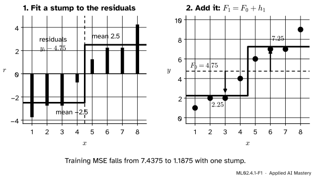
Now fit a regression stump (lesson ML02.1.3) to the residuals instead of to \(y\). It finds that the points left of \(x = 4.5\) sit about \(2.5\) below the mean and the points to the right about \(2.5\) above it. Add that stump to the mean, and the prediction becomes a two-step staircase.
ML02.4.1-F1
One stage of boosting. Left: a stump is fitted to the residuals of the mean, and each leaf predicts the average residual of its points. Right: adding the stump to the mean moves every prediction the way its leaf says.
That is one stage. The new staircase still misses: the point at \(x = 8\) is \(1.75\) above it, the point at \(x = 1\) is \(1.25\) below. These are the new residuals, and the next stump is fitted to them. Each stage looks only at what the model so far gets wrong and nudges the prediction to fix the worst of it. This loop is boosting, and with squared error and regression trees it is the simplest form of gradient boosting.
The contrast with a random forest (ML02.2) is the heart of it. A forest grows deep trees side by side, each on its own sample, and averages them to cut variance. Boosting grows small trees one after another, each depending on all the earlier ones, and adds them to cut bias.
Build it up
Step 1. Start from a constant. The constant with the smallest squared error is the mean, so the stage-0 model is \(F_0(x) = \bar{y} = 4.75\) for every \(x\). Its training mean squared error (MSE) is \(7.4375\), the variance of the targets.
Step 2. Compute the residuals. For each training point, \(r_i^{(0)} = {y_i - F_0(x_i)}\). They are −3.75, −2.75, −2.75, −0.75, 1.25, 2.25, 2.25, 4.25, and they add up to zero.
Step 3. Fit a stump to the residuals. Try every midpoint between neighbouring \(x\) values, put the mean residual of each side in its leaf, and keep the split with the smallest sum of squared errors. Call the fitted stump \(h_1\).
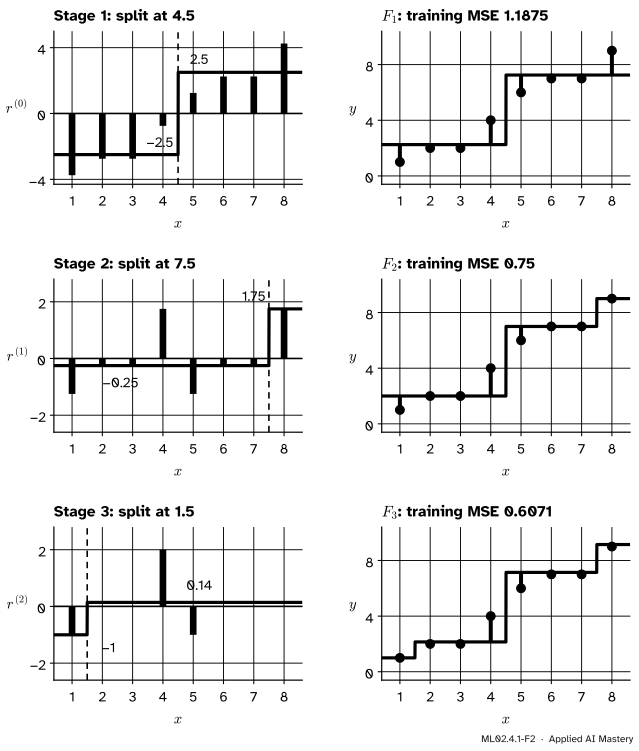
Step 4. Add it and repeat. The new model is \(F_1 = {F_0 + h_1}\). Its residuals are what \(h_1\) could not explain, and the next stump is fitted to them. The figure runs three stages.
ML02.4.1-F2
Three stages, one per row. Each stump (left) is fitted to the residuals the stages before it left, and the staircase (right) gains one step. The training MSE falls from \(1.1875\) to \(0.75\) to \(0.6071\).
Notice what the stumps choose. Stage 2 does not split at \(4.5\) again; it isolates the point at \(x = 8\), which the first staircase underpredicted most. Stage 3 isolates the point at \(x = 1\). Every stage goes after the largest pattern still left in the errors.
The formal statement
NoteDefinition: least-squares boosting with stumps
Given training points \((x_i, y_i)\), \(i = 1, \dots, n\), set \(F_0(x) = \bar{y}\). For each stage \(m = 1, \dots, M\):
compute the residuals \(r_i = y_i - F_{m-1}(x_i)\);
fit a regression stump \(h_m\) to the pairs \((x_i, r_i)\) by least squares;
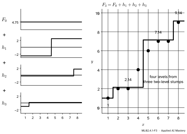
Each \(h_m\) is a step function with one jump, so \(F_M\) is a constant plus \(M\) step functions: a staircase with at most \(M\) jumps. Three two-level stumps can make four levels.
ML02.4.1-F3
The boosted model is a sum. Adding the constant and the three stumps of the worked example gives a staircase with four levels.
Three facts follow, each in a line or two.
Fact 1: a leaf’s best value is the mean of its residuals. For the points in one leaf, the squared error of a constant \(c\) is \({S(c) = \sum (r_i - c)^2}\). Its derivative is \({-2 \sum (r_i - c)}\), which is zero when \({\sum r_i = k\,c}\), where \(k\) is the number of points in the leaf. So \({c = \frac{1}{k} \sum r_i}\), the mean. The same argument with \(r_i\) replaced by \(y_i\) shows that \(F_0 = \bar{y}\).
Fact 2: the training error never goes up. After stage \(m\), each residual is \({r_i - h_m(x_i)}\), so the new sum of squared errors is
A stump whose two leaves both hold \(0\) would leave the residuals unchanged. The fitted stump puts the best constant in each leaf (Fact 1), so it does at least as well as that stump of zeros: \(\text{SSE}_m \le \sum r_i^2 = \text{SSE}_{m-1}\).
Fact 3: the split just used is now worthless. After stage \(m\), the residuals in each leaf of \(h_m\) have mean zero, because their mean was subtracted. Fitting the same split again would put \(0\) in both leaves. That is why stage 2 moves to a new split.
Go deeper: boosting stumps can reach zero training error
With one feature and distinct inputs, a sum of stumps can make any staircase whose jumps sit at the midpoints, and such a staircase can pass through all eight targets. Fact 2 says the training error never rises; in practice it keeps falling. On the eight points it is \(0.0818\) after ten stages and about \(0.001\) after thirty. A model that reaches zero training error has memorised the noise along with the signal, which is why lesson ML02.4.4 stops boosting early.
Worked example
Three stages by hand, with the learning rate \(\cparam{\nu} = 1\).
Stage 1. The residuals of \(F_0 = 4.75\) are (−3.75, −2.75, −2.75, −0.75, 1.25, 2.25, 2.25, 4.25). Try the split at \(4.5\). The left residuals have mean \(-2.5\) and deviations (−1.25, −0.25, −0.25, 1.75), whose squares add to
The right residuals have mean \(2.5\) and the same deviations, so the split’s SSE is \({4.75 + 4.75 = 9.5}\). Every other split does worse; the next best, at \(3.5\), gives \(13.87\). So \(h_1\) is \(-2.5\) for \(x \le 4.5\) and \(2.5\) beyond, \(F_1\) is \(2.25\) then \(7.25\), and the training MSE is \({9.5 / 8 = 1.1875}\).
Stage 2. The new residuals are (−1.25, −0.25, −0.25, 1.75, −1.25, −0.25, −0.25, 1.75). The split at \(4.5\) now scores \(9.5\), no gain at all (Fact 3). The split at \(7.5\) puts seven residuals with mean \(-0.25\) on the left and \(1.75\) alone on the right. The left squares add to \({9.5 - 3.0625 = 6.4375}\), minus \({7 \times 0.0625 = 0.4375}\) for the mean, so the SSE is \(6.0\) and the MSE is \({6 / 8 = 0.75}\).
Stage 3. The residuals are (−1, 0, 0, 2, −1, 0, 0, 0). The split at \(1.5\) isolates the \(-1\) at \(x = 1\); the other seven residuals sum to \(1\), so their leaf holds \({1/7 \approx 0.143}\). Their squares add to \(5\), and the SSE is \({5 - 7 \times (1/7)^2 = 34/7}\), so the MSE is \({34/56 \approx 0.6071}\).
ML02.4.1-F4
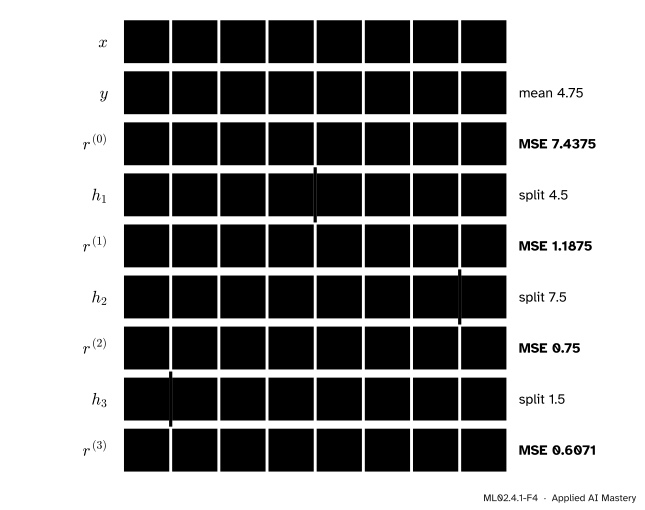
The whole worked example on one card. Each stump row is fitted to the residual row above it, and the residual row below is their difference.
A new input such as \(x = 3.6\) falls in the leaves \(x \le 4.5\), \(x \le 7.5\) and \(x > 1.5\), so \({F_3(3.6)} = 4.75 - 2.5 - 0.25 + 0.143 \approx 2.14\).
Code
First from scratch. The stump finder is the regression-tree split search of lesson ML02.1.3, stopped after one split.
import numpy as npx = np.arange(1.0, 9.0)y = np.array([1, 2, 2, 4, 6, 7, 7, 9], dtype=float)def best_stump(x, r):"""Split at the midpoint with the least squared error; each leaf holds its mean residual.""" values = np.unique(x) best =Nonefor s in (values[:-1] + values[1:]) /2: left = x <= s a, b = r[left].mean(), r[~left].mean() sse = ((r[left] - a) **2).sum() + ((r[~left] - b) **2).sum()if best isNoneor sse < best[3] -1e-12: best = (s, a, b, sse)return bestdef boost(x, y, stages, nu=1.0): f0 = y.mean() pred = np.full(len(y), f0) stumps, mse = [], [np.mean((y - pred) **2)]for _ inrange(stages): s, a, b, _ = best_stump(x, y - pred) # fit to the residuals, not to y stumps.append((s, a, b)) pred = pred + nu * np.where(x <= s, a, b) mse.append(np.mean((y - pred) **2))return f0, stumps, msedef predict(f0, stumps, x_new, nu=1.0):return f0 + nu *sum(np.where(x_new <= s, a, b) for s, a, b in stumps)f0, stumps, mse = boost(x, y, stages=3)print("splits:", [s for s, _, _ in stumps])print("training MSE:", np.round(mse, 4))print("F3 at x = 3.6:", round(float(predict(f0, stumps, np.array(3.6))), 4))
splits: [np.float64(4.5), np.float64(7.5), np.float64(1.5)]
training MSE: [7.4375 1.1875 0.75   0.6071]
F3 at x = 3.6: 2.1429
Now scikit-learn. GradientBoostingRegressor with max_depth=1 grows stumps, and learning_rate=1.0 turns shrinkage off. staged_predict gives the prediction after each stage.
from sklearn.ensemble import GradientBoostingRegressorgbr = GradientBoostingRegressor(n_estimators=3, learning_rate=1.0, max_depth=1)gbr.fit(x.reshape(-1, 1), y)staged_mse = [np.mean((y - p) **2) for p in gbr.staged_predict(x.reshape(-1, 1))]print("library splits:", [float(t.tree_.threshold[0]) for t in gbr.estimators_[:, 0]])print("library MSE:", np.round(staged_mse, 4))
The library takes the same three splits and reaches the same three errors.
Explore
ML02.4-X1
Residual stepper
Press Step on the eight points and check the three training errors of the worked example. Then switch to the noisy sine: with depth-2 trees and a learning rate of 1, watch the training error keep falling while the validation error turns back up.
Pitfalls
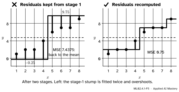
ML02.4.1-F5
Wrong beside right. If the residuals are computed once and never updated, every stage fits the same stump, and two copies of it overshoot all the way back to the error of the mean.
“Compute the residuals once, then fit all the trees to them.”
Each tree must be fitted to the residuals of the model as it stands. Fitted to the stage-0 residuals again, stage 2 picks the split \(4.5\) again and adds another \(\pm 2.5\), giving predictions \(-0.25\) and \(9.75\). The training MSE goes back up to \(7.4375\). Recompute \({r_i = y_i - F_{m-1}(x_i)}\) at every stage.
“Boosting is just bagging with small trees.”
Bagging fits every tree to the same targets on a different resample and averages; the trees do not know about each other. Boosting fits each tree to the errors of all the trees before it and adds them. Averaging the three stumps of the worked example instead of adding them would divide every correction by three, and the stumps of stages 2 and 3 only make sense on top of stage 1.
“The training error keeps falling, so the model keeps improving.”
Fact 2 guarantees the training error never rises, whatever is happening on new data. Boosting keeps fitting finer and finer patterns in the residuals, and after a while those patterns are noise. Watch a validation error, as in the noisy-sine setting of the explorer and in lesson ML02.4.4.
Check yourself
Recall
1. What does the stage-0 model of least-squares boosting predict, and why that value?
Show answer
The mean of the targets, \(\bar{y}\). It is the constant with the smallest sum of squared errors, because the derivative of \({\sum (y_i - c)^2}\) is zero at \({c = \bar{y}}\).
2. At stage \(m\), what is the stump fitted to?
Show answer
The current residuals \({r_i = y_i - F_{m-1}(x_i)}\), paired with the inputs \(x_i\).
3. On the eight points with \(\cparam{\nu} = 1\), what are the training MSEs after one, two and three stages?
Show answer
\(1.1875\), \(0.75\) and \(0.6071\) (that is, \(34/56\)), with splits at \(4.5\), \(7.5\) and \(1.5\).
4. Why can the training error of least-squares boosting never go up from one stage to the next?
Show answer
Leaves holding \(0\) would leave the residuals unchanged, and the fitted stump puts the best constant (the mean residual) in each leaf, so its squared error is at most the old one.
5. Why does stage 2 not reuse the split at \(4.5\)?
Show answer
After stage 1 the residuals in each of its leaves have mean zero, so the same split would put \(0\) in both leaves and gain nothing.
Exercises
1.★ Using the stumps of the worked example, compute \(F_1\), \(F_2\) and \(F_3\) at the new input \(x = 7.8\).
2.★★ Run one stage of boosting by hand on four points \(x = 1, 2, 3, 4\) with targets \(y = (3, 5, 4, 12)\). Give \(F_0\), the best split, the two leaf values, \(F_1\) and its training MSE.
Show solution
\(F_0 = 24/4 = 6\), so the residuals are (−3, −1, −2, 6) and the MSE of \(F_0\) is \({(9 + 1 + 4 + 36)/4 = 12.5}\). Split at \(1.5\): leaves \(-3\) and \({(-1 - 2 + 6)/3 = 1}\); the right deviations are \((-2, -3, 5)\), SSE \({4 + 9 + 25 = 38}\). Split at \(2.5\): leaves \(-2\) and \(2\); deviations \((-1, 1)\) and \((-4, 4)\), SSE \(34\). Split at \(3.5\): leaves \(-2\) and \(6\); the left deviations are \((-1, 1, 0)\), SSE \(2\). The best split is \(3.5\), so \(F_1 = (4, 4, 4, 12)\) and the training MSE is \({2/4 = 0.5}\).
3.★★★ Show that after any stage of least-squares boosting, the training residuals add up to zero. Then use it to explain why \(F_m\) has the same mean over the training points as \(y\).
Show solution
At stage 0 the residuals \({y_i - \bar{y}}\) add up to \({n\bar{y} - n\bar{y} = 0}\). Suppose the residuals \(r_i\) before stage \(m\) add up to zero. The stump subtracts the mean residual of each leaf from the residuals in that leaf, so within each leaf the new residuals add up to zero, and so does their total. (With a learning rate \(\cparam{\nu}\), each leaf’s residuals then add up to \({(1 - \cparam{\nu})}\) times their old sum, and those old sums still add up to zero.) By induction the residuals add up to zero after every stage. Then \({\sum F_m(x_i) = \sum y_i - \sum r_i = \sum y_i}\), so the mean prediction equals \(\bar{y}\).
Summary card
Each stage fits a small tree to what the model still gets wrong, and adds it.
ML02.4.1-F1
Fit the residuals, then add.
Start.\(F_0 = \bar{y}\).
Stage \(m\).\({r_i = y_i - F_{m-1}(x_i)}\); fit \(h_m\) to \((x_i, r_i)\); \({F_m = F_{m-1} + \cparam{\nu}\, h_m}\).
Leaves. Each leaf holds the mean residual of its points.
Sources. Each was opened and checked against this lesson on 15 November 2026.
Trevor Hastie, Robert Tibshirani and Jerome Friedman, The Elements of Statistical Learning, 2nd edition, 12th printing. Section 10.10.2 notes that for squared-error loss the negative gradient “is just the ordinary residual”, so fitting a tree to it is “standard least-squares boosting”; Algorithm 10.3 (page 361) starts from the best constant and adds one tree per iteration. Section 10.12 notes that each iteration usually reduces the training risk, which can be made arbitrarily small.
Gareth James, Daniela Witten, Trevor Hastie and Robert Tibshirani, An Introduction to Statistical Learning, 2nd edition, Section 8.2.3. Algorithm 8.2 fits each tree to the current residuals and adds a shrunken copy of it, and the text explains that boosting “learns slowly” and that each tree depends on those grown before.
scikit-learn developers, User Guide 1.11.1.2, version 1.9.1. The additive form \({F_m = F_{m-1} + h_m}\) of GradientBoostingRegressor, with staged_predict for the prediction after each stage.