Bin each feature once, and the search for the best split becomes a pass over a few hundred bin sums of g and h, with one child’s histogram got free by subtraction. Then grow the most promising leaf first, and let missing values learn which way to go.
ML02.5.2L2 Intermediate30 minIn review (what this means)
The maths and code on this page are checked by automated tests on every change, but an independent reader has not signed it off yet. Spot a mistake or a confusing step? Tell us.
Build a gradient histogram for one feature and find the best split by scanning its bin edges.
Derive the subtraction trick and compare the cost of the histogram search with the sorted search.
Contrast level-wise and leaf-wise growth on a small example and say why leaf-wise growth needs a limit.
Explain how a split learns a default direction for missing values, and use max_bins, max_leaf_nodes and NaN inputs in HistGradientBoosting.
The question
A bank scores ten million loans with two hundred features. The split finder of the last lesson sorts every feature and tries every cut, at every node of every tree of every stage: about ten million candidates per feature per node. LightGBM looks at no more than 255 bins. How can it throw away almost every threshold and still find good splits, and what does it do with the time it saves?
From the last lesson
1. What is the best weight of a leaf whose gradients sum to \(G\) and Hessians to \(H\)?
Show answer
\(w = {-G/(H + \lambda)}\).
2. What must the gain of a split exceed for the split to be made?
Show answer
Zero, after the fee \(\gamma\) has been taken off. Equivalently, the gain before the fee, half of \({G_L^2/(H_L + \lambda)} + {G_R^2/(H_R + \lambda)} - {G^2/(H + \lambda)}\), must exceed \(\gamma\).
Intuition
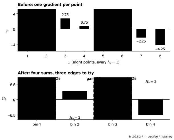
The gain needs only two numbers from each side of a cut: the sums \(G\) and \(H\). So the points themselves do not matter, only their sums. Put the values of a feature into a few bins, once, before training starts. To score a node, add up \(g\) and \(h\) in each bin, then slide the cut along the bin edges, carrying running sums.
ML02.5.2-F1
The eight points of the last lesson in four bins of two. Eight gradients become four bin sums, and seven candidate thresholds become three. The best of them, \(4.5\), is the same split as before, with gain \(25\).
That is the histogram algorithm. A histogram is the list of bin sums \({(G_b, H_b)}\) of one feature in one node: one pass over the rows to build, one step per bin to scan.
Build it up
Step 1. Bin once. For each feature, choose at most \(B\) bins (LightGBM and scikit-learn use \(B = 255\) by default) from quantiles of the training values, so that each bin holds about the same number of rows. Replace every value by its bin number, an integer below 256 that fits in one byte.
Step 2. Build a node’s histogram. For every row in the node, add its \(g_i\) and \(h_i\) to its bin. With \(n\) rows in the node this is \(n\) additions per feature.
Step 3. Scan the edges. Walk the bins from left to right with running sums \(G_L\) and \(H_L\). At each edge, \(G_R = G - G_L\) and \(H_R = H - H_L\), and the gain formula does the rest.
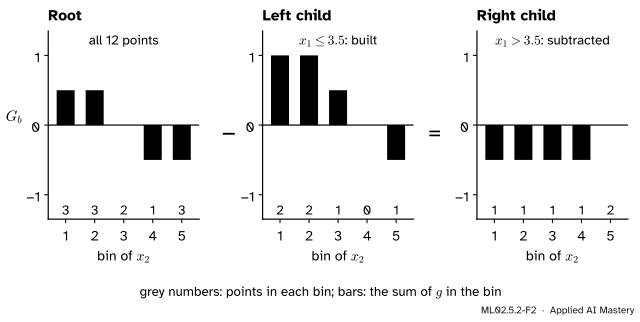
Step 4. Get one child free. After a split, each child needs its own histogram. But a bin of the parent holds exactly the rows of that bin in the left child plus those in the right child, so the right child’s histogram is the parent’s minus the left child’s, bin by bin. Build the smaller child by adding its rows; get the larger one by subtraction.
ML02.5.2-F2
The subtraction trick on the course’s twelve points, at the start of boosting with the log loss (\(p = 0.5\), so \(g = 0.5\) for class 0 and \(-0.5\) for class 1). After the root split \(x_1 \le 3.5\), the histogram of \(x_2\) in the right child is the root’s minus the left child’s.
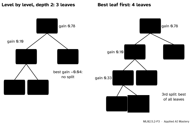
Step 5. Grow the best leaf first. XGBoost grows a tree level-wise: it splits every leaf of one depth before going deeper. LightGBM grows it leaf-wise, or best-first: of all current leaves it splits the one whose best split has the largest gain, and stops at a set number of leaves.
ML02.5.2-F3
Two ways to grow a tree on the dozen of the worked example. Level by level to depth 2, the right child has no split worth making and the tree stops at three leaves. Best leaf first, with four leaves allowed, keeps going where the gain is largest, here one level deeper, and ends with a leaf holding a single point.
The formal statement
NoteDefinition: gradient histogram
For one feature with bins \(b = 1, \dots, B\) and the rows \(I\) of a node,
The cut after bin \(k\) has \(G_L = G_1 + \dots + G_k\) and \(H_L = H_1 + \dots + H_k\).
Same gain, fewer cuts. The cut after bin \(k\) sends exactly the rows of bins \(1\) to \(k\) to the left. Their gradients add to \(G_1 + \dots + G_k\), because addition can be regrouped bin by bin. So the gain at a bin edge is exactly the gain of the last lesson for that threshold. Binning does not approximate the gain; it only restricts the thresholds to the \(B - 1\) bin edges.
The subtraction identity. Every row of the parent lies in exactly one child, so for each bin
and the same for \(H_b\). Rearranged, \({G_b^{\text{right}} = G_b^{\text{parent}} - G_b^{\text{left}}}\): \(B\) subtractions instead of a pass over the right child’s rows.
Cost. Take a node with \(n\) rows and \(d\) features. Over a whole level of a tree the nodes together hold every row once.
Step
Sorted search
Histograms
Before training
sort each feature
bin each feature
Per node, gather
–
\(n d\) additions
Per node, scan
\(n d\) cuts
\(B d\) cuts
Ke et al. (Section 2.1) put the cost of the histogram algorithm at \({O(\#\text{data} \times
\#\text{feature})}\) for building and \({O(\#\text{bin} \times \#\text{feature})}\) for split finding, with building the larger part. The subtraction trick at least halves the building: only the smaller child, at most \(n/2\) rows, is ever built.
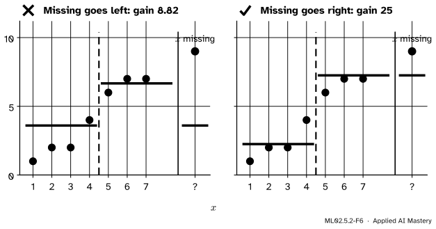
Missing values. A row whose feature is missing has no bin on the number line. XGBoost (Section 3.4 of Chen and Guestrin) and scikit-learn try both directions for each cut: once with the missing rows’ sums \({(G_?, H_?)}\) added to the left, once to the right, and keep whichever gives the larger gain. The winning side is stored with the split as its default direction.
ML02.5.2-F6
A missing value learns its direction. The point \(y = 9\) has no \(x\). Sent left, its large residual spoils the left leaf and the gain is \(8.82\); sent right, the gain is \(25\). So this split sends missing values right.
Leaf-wise growth. With \(L\) leaves allowed, level-wise growth to depth \(D\) needs \(L = 2^D\) leaves to fill the last level, while leaf-wise growth can reach depth \(L - 1\) along one path. The LightGBM documentation says that, for the same number of leaves, leaf-wise growth tends to reach a lower loss, and warns that it may overfit when the data are few; max_depth and a minimum number of rows per leaf then rein it in.
Go deeper: two more ideas from the LightGBM paper
Gradient-based one-side sampling (GOSS, Section 3). Rows with small \(\abs{g_i}\) are already fitted well. Keep the top fraction \(a\) of rows by \(\abs{g_i}\), sample a fraction \(b\) of all rows from the rest, and multiply the sampled rows’ \(g\) and \(h\) by \({(1 - a)/b}\). The rest hold \({(1 - a)n}\) rows of which \(bn\) are drawn, so each drawn row stands for \({(1 - a)/b}\) of them, and the expected sums \(G\) and \(H\) do not change.
Exclusive feature bundling (EFB, Section 4). In sparse data many features are never non-zero in the same row, such as the columns of a one-hot code. Such features can share one column: give each its own range of bin numbers and add the offsets. Histograms are then built per bundle instead of per feature. Finding the fewest bundles is NP-hard (their Theorem 4.1), so a greedy method is used.
Worked example
The dozen. Twelve points along one feature, \(x = 1, \dots, 12\), with labels \(y\) and the probabilities \(p\) that the model so far gives them, made up for this module:
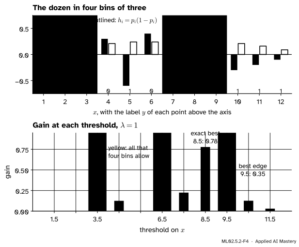
The other edges give \(0.021\) (at \(3.5\)) and \(0.014\) (at \(6.5\)), so the histogram search splits at \(9.5\), with weights \(-1.3/2.83 = -0.459\) and \(0.6/1.46 = 0.411\).
The exact search tries all eleven thresholds and finds \(8.5\), with \(G_L = 1.7\), \(H_L = 1.59\), \(G_R = -1.0\), \(H_R = 0.70\) and a gain of \(0.778\), more than twice as large.
ML02.5.2-F4
The trace. Top: gradients (filled) and Hessians (outlined), with the four bins shaded. Bottom: the gain at every threshold. Four bins allow only the three yellow thresholds, and miss the best.
Four bins for twelve points are very coarse, and here they cost half the gain. With 255 bins little is lost; scikit-learn even notes that fewer bins act as a form of regularisation.
Growing. Level by level, to depth 2: the root splits at \(8.5\). Its left child, points 1 to 8, splits at \(5.5\) (gain \(0.103\)); its right child has no positive gain (the best is \(-0.038\)) and stays a leaf. Best leaf first, with four leaves allowed, makes the same two splits, then splits points 1 to 5 at \(4.5\) (gain \(0.332\)), and the single point \(x = 5\) gets a leaf of its own.
Code
First the histogram search, from scratch, on the dozen.
import numpy as npx = np.arange(1.0, 13.0)y = np.array([0, 0, 0, 0, 1, 0, 0, 0, 1, 1, 1, 1], dtype=float)p = np.array([0.1, 0.2, 0.2, 0.3, 0.4, 0.4, 0.5, 0.6, 0.6, 0.7, 0.8, 0.9])g, h = p - y, p * (1- p)lam =1.0def gain(GL, HL, GR, HR):return0.5* (GL**2/ (HL + lam) + GR**2/ (HR + lam) - (GL + GR)**2/ (HL + HR + lam))def bin_edges(values, n_bins):"""Inner edges at quantiles, so that bins hold about equal numbers of rows."""return np.quantile(values, np.arange(1, n_bins) / n_bins, method="midpoint")def histogram(bins, g, h, n_bins):return np.bincount(bins, weights=g, minlength=n_bins), np.bincount(bins, weights=h, minlength=n_bins)def best_edge(Gb, Hb, edges): GL, HL = np.cumsum(Gb)[:-1], np.cumsum(Hb)[:-1] gains = gain(GL, HL, Gb.sum() - GL, Hb.sum() - HL) k =int(np.argmax(gains))returnfloat(edges[k]), float(gains[k])edges = bin_edges(x, 4)bins = np.searchsorted(edges, x) # bin number of every row: 0, 1, 2 or 3Gb, Hb = histogram(bins, g, h, 4)print("edges", edges, " G_b", np.round(Gb, 2), " H_b", np.round(Hb, 2))print("histogram search:", best_edge(Gb, Hb, edges))exact = best_edge(g, h, (x[:-1] + x[1:]) /2) # one bin per point is the exact searchprint("exact search:", exact)
The library. HistGradientBoostingRegressor bins with max_bins, grows best-first up to max_leaf_nodes leaves, and learns a direction for missing values. On the eight points with one stump, three bins move the cut away from \(4.5\); four bins keep it.
import osos.environ.setdefault("OMP_NUM_THREADS", "1") # one thread is faster on data this smallfrom sklearn.ensemble import HistGradientBoostingRegressorx8 = np.arange(1.0, 9.0).reshape(-1, 1)y8 = np.array([1.0, 2.0, 2.0, 4.0, 6.0, 7.0, 7.0, 9.0])stump =dict(max_iter=1, learning_rate=1.0, max_leaf_nodes=2, min_samples_leaf=1, early_stopping=False)for n_bins in (3, 4): model = HistGradientBoostingRegressor(max_bins=n_bins, **stump).fit(x8, y8)print(f"max_bins = {n_bins}: leaf values {np.unique(model.predict(x8).round(4))}")x8_holes = x8.copy()x8_holes[7] = np.nan # the last point's x is missingmodel = HistGradientBoostingRegressor(**stump).fit(x8_holes, y8)print("a missing x is predicted", model.predict([[np.nan]]))
max_bins = 3: leaf values [1.6667 6.6   ]
max_bins = 4: leaf values [2.25 7.25]
a missing x is predicted [7.25]
With three bins the edges fall between 3 and 4 and between 6 and 7, so the best cut available is the one before \(x = 4\), giving leaves \(5/3\) and \(6.6\). And the missing \(x\) goes right, to \(7.25\), as in the figure. Last, a real table with holes: knock out a tenth of the entries of load_breast_cancer at random and fit the classifier without imputing anything.
from sklearn.datasets import load_breast_cancerfrom sklearn.ensemble import HistGradientBoostingClassifierfrom sklearn.model_selection import train_test_splitX, y_bc = load_breast_cancer(return_X_y=True)X_holes = X.copy()X_holes[np.random.default_rng(0).random(X.shape) <0.1] = np.nanprint(f"rows with at least one hole: {np.isnan(X_holes).any(axis=1).mean():.0%}")X_tr, X_te, y_tr, y_te = train_test_split(X_holes, y_bc, test_size=0.25, random_state=0, stratify=y_bc)clf = HistGradientBoostingClassifier(max_bins=255, max_leaf_nodes=31, random_state=0).fit(X_tr, y_tr)print(f"test accuracy with holes: {clf.score(X_te, y_te):.3f}")
rows with at least one hole: 96%
test accuracy with holes: 0.930
Dropping incomplete rows would throw away nearly all the data. The model uses all of it, holes included, and scores about 93 percent on the test rows.
Explore
ML02.5-X1
Split-gain calculator
Drag the dashed threshold, or use its slider, and watch \(G\), \(H\), the two leaf weights and the gain. Then raise \(\lambda\) and \(\gamma\), and lower the number of bins.
Set the bins to 4 and the best cut jumps from \(8.5\) to \(9.5\). Raise \(\gamma\) above the best gain and no split pays.
Pitfalls
ML02.5.2-F5
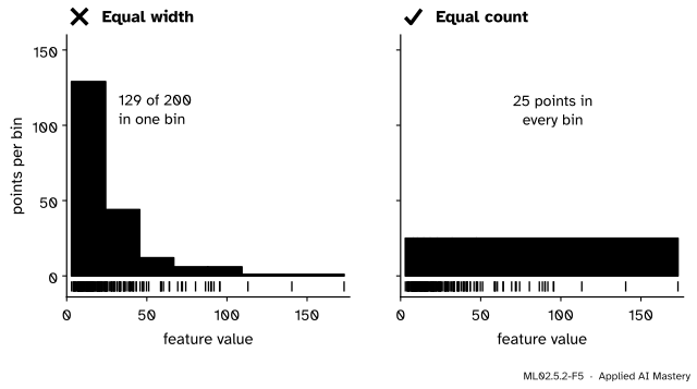
Wrong beside right, on 200 values of a skewed feature. Left: bins of equal width put most points in one bin, so the dense region gets almost no thresholds. Right: bins at quantiles hold 25 points each, so the thresholds follow the data.
“Bins should all be the same width.”
On a skewed feature, such as an income, equal widths waste bins on the empty tail and lump the crowd together. Quantile bins put the thresholds where the rows are.
“Binning makes the gain approximate.”
The gain at a bin edge is exact; binning only restricts which thresholds are tried.
“Leaf-wise growth is simply better, so leave the tree unlimited.”
For a given number of leaves it usually reaches a lower training loss, and on a small dataset that means overfitting: on the dozen its fourth leaf held one point. Limit the number of leaves (num_leaves, max_leaf_nodes), the depth, and the rows per leaf (min_data_in_leaf, min_samples_leaf, 20 by default in both libraries).
Check yourself
Recall
1. What two numbers does a gradient histogram store for each bin?
Show answer
The sum of the gradients \(G_b\) and the sum of the Hessians \(H_b\) of the node’s rows in that bin.
2. Why is the gain at a bin edge exact?
Show answer
The cut sends exactly the rows of the bins on its left to the left child, and their \(g\) and \(h\) add up bin by bin to the same \(G_L\) and \(H_L\) as in the sorted search.
3. State the subtraction trick.
Show answer
For every bin, the right child’s histogram equals the parent’s minus the left child’s, because every row of the parent is in exactly one child. Build the smaller child; subtract for the other.
4. How does leaf-wise growth choose the next split?
Show answer
It looks at the best split of every current leaf and makes the one with the largest gain, wherever it is in the tree, until the number of leaves reaches its limit.
5. How is the default direction for missing values chosen?
Show answer
For each candidate cut the gain is computed twice, with the missing rows’ sums added to the left and to the right; the larger decides, and that side is stored with the split.
Exercises
1.★ A node’s histogram for one feature has \(G_b = {(2, -1, -3)}\) and \(H_b = {(1, 1, 2)}\), and \(\lambda = 0\). Find the gain at both edges.
Show solution
In total \(G = -2\) and \(H = 4\), so the parent term is \({(-2)^2/4} = 1\). First edge: \(G_L = 2\), \(H_L = 1\), \(G_R = -4\), \(H_R = 3\), gain \({\tfrac12(4 + 16/3 - 1)} = 4.17\). Second edge: \(G_L = 1\), \(H_L = 2\), \(G_R = -3\), \(H_R = 2\), gain \({\tfrac12(0.5 + 4.5 - 1)} = 2\). The first edge wins.
2.★★ In the eight points, suppose instead that the first point (\(y = 1\)) has its \(x\) missing. At the threshold \(4.5\) with \(\lambda = 0\), which way should it go, and with what gain?
Show solution
The point has \(g = 3.75\). The known rows left of \(4.5\) are \(x = 2, 3, 4\), with \(G = 2.75 + 2.75 + 0.75 = 6.25\) and \(H = 3\); right of it, \(G = -10\) and \(H = 4\).
(The parent term is \(0\) because \(G = 0\).) It goes left, with gain \(25\).
3.★★★ GOSS keeps the top \(a n\) rows by \(\abs{g_i}\) and draws \(b n\) of the other \({(1 - a)n}\) rows at random, each equally likely. Show that multiplying each drawn row’s \(g_i\) by \({(1 - a)/b}\) makes the expected sum of the drawn rows’ gradients equal to the sum over all the other rows.
Show solution
Let \(R\) be the set of the other rows, with \(\abs{R} = {(1 - a)n}\). Drawing \(bn\) of them without favouring any, each row of \(R\) is drawn with probability \({bn / ((1 - a)n)} = {b/(1 - a)}\). Write \(D_i = 1\) if row \(i\) is drawn and \(0\) otherwise. Then
Cost per node.\(n d\) to build, \(B d\) to scan, instead of \(n d\) cuts.
Leaf-wise. Split the best leaf anywhere; limit leaves, depth and rows per leaf.
Missing values. Try both sides; keep the better as the default direction.
Sources and next steps
Sources. Each was opened and checked against this lesson on 15 November 2026.
Guolin Ke, Qi Meng, Thomas Finley and others, LightGBM: A Highly Efficient Gradient Boosting Decision Tree, NeurIPS 2017. Section 2.1 (the pre-sorted and histogram algorithms and their costs), Section 3 (GOSS, with the top \(a\) and the factor \({(1 - a)/b}\)) and Section 4 (EFB and Theorem 4.1).
LightGBM developers, Features, LightGBM documentation. Histogram subtraction from the parent and the neighbour, leaf-wise growth that picks the leaf with the largest loss reduction, its lower loss for a fixed number of leaves and its risk of overfitting on small data, and max_depth as the limit.
scikit-learn developers, Ensembles, Section 1.11.1.1, scikit-learn 1.9 User Guide. Binning with max_bins (255 by default; fewer bins regularise), inspiration from LightGBM, and missing values sent left or right by the gain.