Describe each class as a cloud with a centre and a covariance matrix. Read the cloud’s tilted ellipses off the eigenvectors, measure distance in the cloud’s own units with the Mahalanobis distance, and fit each class of the twelve points by maximum likelihood.
ML02.9.1L2 Intermediate25 minIn review (what this means)
The maths and code on this page are checked by automated tests on every change, but an independent reader has not signed it off yet. Spot a mistake or a confusing step? Tell us.
Write the density of a two-dimensional Gaussian with mean vector and covariance matrix, and explain what each part does.
Draw the contour ellipses of a Gaussian from the eigenvectors and eigenvalues of its covariance matrix.
Compute the Mahalanobis distance of a point from a class and explain why it can disagree with the ordinary distance.
Fit a class mean and covariance by maximum likelihood by hand, and recognise Gaussian naive Bayes as the case of diagonal covariances.
The question
Gaussian naive Bayes saw class 0 of the twelve points as a round cloud. But look at the points: when \(x_1\) is large, \(x_2\) tends to be large too, so the cloud leans along the diagonal. How do we describe a cloud that leans, and what does it then mean for a new point to be “close” to a class?
Intuition
Think of each class as a cloud of points. A Gaussian cloud needs only two things: a centre, the mean vector\(\vect{\mu}\), and a shape, the covariance matrix\(\mat{\Sigma}\). Its density falls off from the centre in rings, and in two dimensions every ring is an ellipse.
ML02.9.1-F1
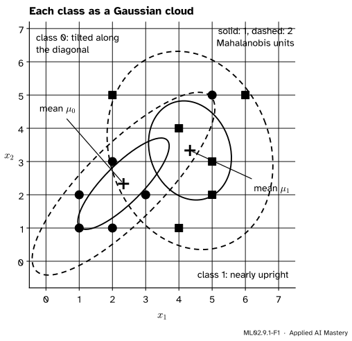
Each class of the twelve points as a Gaussian cloud with its own mean and covariance. Class 0 leans along the diagonal; class 1 is nearly upright. The ellipses are contours of equal density.
The lean is the new ingredient. In Gaussian naive Bayes each feature had its own bell, so the ellipses could only stand straight. A covariance matrix adds one number per pair of features that says how they move together, and that number tilts the ellipse.
Once a class is a cloud, “close to the class” means “inside a small ellipse”, not “inside a small circle”. A point on the long axis of the cigar is typical even when it is some way from the centre; a point the same distance away across the narrow axis is not.
Build it up
Step 1. Two features, five numbers. A cloud in the plane has a mean \({\vect{\mu} = (\mu_1, \mu_2)}\) and a covariance matrix with the two variances on its diagonal and the covariance off it (M06.10):
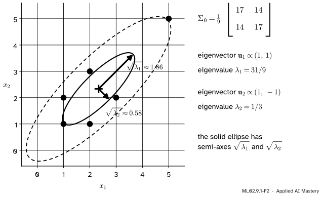
Step 2. The ellipse lies along the eigenvectors.\(\mat{\Sigma}\) is symmetric, so it has two perpendicular eigenvectors \(\vect{u}_1, \vect{u}_2\) with eigenvalues \({\lambda_1 \ge \lambda_2 > 0}\) (the spectral theorem, M03.3). Along \(\vect{u}_i\) the cloud has variance \(\lambda_i\). The ellipse’s axes point along the eigenvectors, and its semi-axes are \(\sqrt{\lambda_1}\) and \(\sqrt{\lambda_2}\).
ML02.9.1-F2
The covariance matrix of class 0 and its ellipse. The long axis is the eigenvector \((1, 1)\) with eigenvalue \(31/9\); the short axis is \((1, -1)\) with eigenvalue \(1/3\).
Step 3. Measure distance in the cloud’s own units. Along the long axis one unit of the cloud is \({\sqrt{31/9} \approx 1.86}\); along the short axis it is only \({\sqrt{1/3} \approx 0.58}\). Count how many of these units a point is from the centre, along each axis, and combine them by Pythagoras. That count is the Mahalanobis distance\(\Delta\).
Step 4. The density depends on \(\Delta\) alone. A Gaussian cloud is highest at its centre and falls off as \({e^{-\Delta^2/2}}\). Points with the same \(\Delta\) have the same density, which is why the contours are the ellipses \({\Delta = 1}\), \({\Delta = 2}\), and so on.
The formal statement
NoteDefinition: the multivariate Gaussian
A random vector \(\vect{x}\) in \(\R^d\) has the Gaussian (normal) distribution \({N(\vect{\mu}, \mat{\Sigma})}\), with mean \(\vect{\mu}\) and a symmetric positive definite covariance matrix \(\mat{\Sigma}\), when its density is
For \({d = 2}\) the constant in front is \({1/(2\pi\sqrt{\det \mat{\Sigma}})}\). This lesson needs the density only this far; M07.3 treats the Gaussian in full.
Why the contours are ellipses. Write the spectral decomposition \({\mat{\Sigma} = \lambda_1 \vect{u}_1\vect{u}_1\T + \lambda_2 \vect{u}_2\vect{u}_2\T}\). The inverse has the same eigenvectors and the reciprocal eigenvalues:
(Multiply the two sums: the cross terms vanish because \({\vect{u}_1\T\vect{u}_2 = 0}\), and what is left is \({\vect{u}_1\vect{u}_1\T + \vect{u}_2\vect{u}_2\T}\), the identity.) Put \({\vect{v} = \vect{x} - \vect{\mu}}\) into \(\Delta^2\):
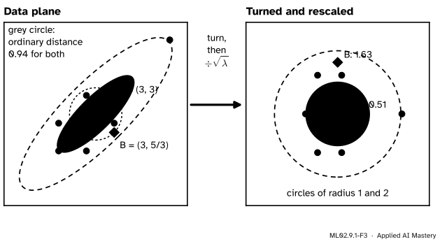
with \({z_i = \vect{u}_i\T\vect{v} / \sqrt{\lambda_i}}\). In words: turn the plane so that the eigenvectors become the axes (that gives \({\vect{u}_i\T\vect{v}}\)), then divide each coordinate by its standard deviation \(\sqrt{\lambda_i}\). In the new coordinates \({\Delta = c}\) is a circle of radius \(c\); back in the plane it is an ellipse with semi-axes \({c\sqrt{\lambda_1}}\) and \({c\sqrt{\lambda_2}}\).
ML02.9.1-F3
The Mahalanobis distance is the ordinary distance after the cloud is made round. \(A\) and \(B\) are equally far from the mean in centimetres, but \(A\) is half a unit out and \(B\) more than one and a half.
In the round coordinates the cloud is two independent standard bells, and a short calculation in polar coordinates (exercise 3) shows that a fraction \({1 - e^{-c^2/2}}\) of the cloud lies inside \({\Delta = c}\): 39% inside the solid ellipse and 86% inside the dashed one.
Fitting a class. For the \(n_k\) training points of class \(k\), the maximum-likelihood estimates are the class mean and the average outer product of the deviations, dividing by \(n_k\) as in S02.3.3:
Entry \({(j, l)}\) of \(\hat{\mat{\Sigma}}_k\) is the average of \({(x_{ij} - \hat\mu_{kj})(x_{il} - \hat\mu_{kl})}\): the variance of feature \(j\) when \({j = l}\) and the covariance of the pair otherwise.
Go deeper: why these are the maximum-likelihood estimates
Write \({\mat{\Lambda} = \mat{\Sigma}^{-1}}\) and drop constants. The log-likelihood of the class is
The mean. The gradient of the sum with respect to \(\vect{\mu}\) is \({-\sum_i \mat{\Lambda}(\vect{x}_i - \vect{\mu})}\) (M05.7.1). It is zero when \({\sum_i (\vect{x}_i - \vect{\mu}) = \vect{0}}\), because \(\mat{\Lambda}\) is invertible, so \({\vect{\mu} = \tfrac{1}{n_k}\sum_i \vect{x}_i}\).
The covariance. A number equals its own trace, and \({\operatorname{tr}(\mat{A}\mat{B}) = \operatorname{tr}(\mat{B}\mat{A})}\), so each quadratic term is \({\operatorname{tr}(\mat{\Lambda}\,\vect{v}_i\vect{v}_i\T)}\) with \({\vect{v}_i = \vect{x}_i - \hat{\vect{\mu}}}\). Summing, \({\ell = \tfrac{n_k}{2}\ln\det\mat{\Lambda} - \tfrac12\operatorname{tr}(\mat{\Lambda}\mat{S})}\) with \({\mat{S} = \sum_i \vect{v}_i\vect{v}_i\T}\). The derivative of \({\ln\det\mat{\Lambda}}\) is \({\mat{\Lambda}^{-1}}\) (M05.7.4) and that of \({\operatorname{tr}(\mat{\Lambda}\mat{S})}\) is \(\mat{S}\), so setting the derivative to zero gives \({\tfrac{n_k}{2}\mat{\Lambda}^{-1} = \tfrac12\mat{S}}\), that is \({\mat{\Sigma} = \mat{S}/n_k}\).
Gaussian naive Bayes is the diagonal case. If \(\mat{\Sigma}\) is diagonal, with variances \(\sigma_1^2\) and \(\sigma_2^2\), then \({\det\mat{\Sigma} = \sigma_1^2\sigma_2^2}\) and \({\Delta^2 = (x_1 - \mu_1)^2/\sigma_1^2 + (x_2 - \mu_2)^2/\sigma_2^2}\). The exponential of a sum is a product, so the density splits into two one-feature bells:
That is exactly the model of ML02.6.4. So Gaussian naive Bayes is this lesson’s model with every covariance forced to zero.
The generative recipe. As in ML02.6.1, fit a cloud \({N(\hat{\vect{\mu}}_k, \hat{\mat{\Sigma}}_k)}\) and a prior \(\pi_k\) for each class, and turn them into a posterior with Bayes’ rule:
The next two lessons turn this recipe into two classifiers: one where all classes share a covariance (LDA), and one where each keeps its own (QDA).
Worked example
Fit class 0 of the twelve points, find its ellipse, and measure how typical \(A = (3, 3)\) and \(B = (3, 5/3)\) are.
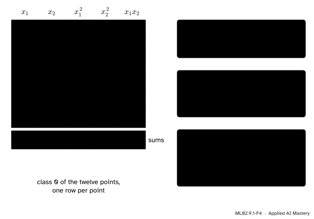
Fit. The six points of class 0 are (1, 1), (2, 1), (1, 2), (2, 3), (3, 2) and (5, 5). Five column sums are all we need.
ML02.9.1-F4
The worked example as a table. Each estimate is an average of a column minus a product of means.
The mean of each feature is \({14/6 = 7/3}\). Each variance is the mean square minus the squared mean, \({44/6 - 49/9 = 17/9}\), and the covariance is the mean product minus the product of means, \({42/6 - 49/9 = 14/9}\). So
The correlation is \({(14/9)/(17/9) = 14/17 = 0.82}\): a strong lean.
Eigenvalues. Solve \({(17/9 - \lambda)^2 = (14/9)^2}\), so \({17/9 - \lambda = \pm 14/9}\) and \({\lambda = 31/9}\) or \({3/9 = 1/3}\). For \({\lambda_1 = 31/9}\) the eigenvector is \({(1, 1)}\), for \({\lambda_2 = 1/3}\) it is \({(1, -1)}\). As unit vectors, \({\vect{u}_1 = (1, 1)/\sqrt{2}}\) and \({\vect{u}_2 = (1, -1)/\sqrt{2}}\).
Point A.\({A - \hat{\vect{\mu}}_0 = (2/3, 2/3)}\), which lies along \(\vect{u}_1\) with length \({2\sqrt{2}/3 = 0.943}\). So \({z_1 = 0.943/\sqrt{31/9}}\) and \({z_2 = 0}\):
Densities.\({\det\hat{\mat{\Sigma}}_0 = (17^2 - 14^2)/81 = 31/27}\), so the peak height is \({1/(2\pi\sqrt{31/27}) = 0.1485}\). At \(A\) the density is \({0.1485\,e^{-4/31} = 0.1306}\); at \(B\) it is \({0.1485\,e^{-4/3} = 0.0392}\), less than a third as high, although both points are 0.943 from the mean.
Code
From scratch with NumPy, then checked against SciPy’s Gaussian density.
import numpy as npfrom scipy.stats import multivariate_normalX = np.array([(1, 1), (2, 1), (1, 2), (2, 3), (3, 2), (5, 5), (4, 1), (5, 2), (5, 3), (4, 4), (2, 5), (6, 5)], dtype=float)y = np.array([0] *6+ [1] *6)def fit_class(Xk): mu = Xk.mean(axis=0) D = Xk - mureturn mu, D.T @ D /len(Xk) # divide by n_k: maximum likelihooddef mahalanobis2(x, mu, Sigma): v = x - mureturn v @ np.linalg.solve(Sigma, v)def density(x, mu, Sigma): d =len(mu)return np.exp(-0.5* mahalanobis2(x, mu, Sigma)) / np.sqrt((2* np.pi) ** d * np.linalg.det(Sigma))mu0, S0 = fit_class(X[y ==0])mu1, S1 = fit_class(X[y ==1])lam, U = np.linalg.eigh(S0) # eigenvalues in increasing orderprint("class 0: mean", mu0.round(4), " covariance x 9:", (9* S0).round(4).tolist())print("eigenvalues x 9:", (9* lam).round(4))A, B = np.array([3.0, 3.0]), np.array([3.0, 5/3])for name, p in (("A", A), ("B", B)):print(f"{name}: distance {np.linalg.norm(p - mu0):.3f}, Mahalanobis {np.sqrt(mahalanobis2(p, mu0, S0)):.3f}, "f"density {density(p, mu0, S0):.4f}")print("SciPy at A:", round(multivariate_normal(mu0, S0).pdf(A), 4))
class 0: mean [2.3333 2.3333]  covariance x 9: [[17.0, 14.0], [14.0, 17.0]]
eigenvalues x 9: [ 3. 31.]
A: distance 0.943, Mahalanobis 0.508, density 0.1306
B: distance 0.943, Mahalanobis 1.633, density 0.0392
SciPy at A: 0.1306
Now the generative recipe with equal priors. Each class keeps its own covariance; for comparison, Gaussian naive Bayes keeps only the diagonal.
def posterior1(x, covs): a, b = density(x, mu0, covs[0]), density(x, mu1, covs[1])return b / (a + b) # equal priors cancelfull = (S0, S1)diagonal = (np.diag(np.diag(S0)), np.diag(np.diag(S1)))print(f"P(class 1 | (3, 3)): full covariances {posterior1(A, full):.3f}, diagonal only {posterior1(A, diagonal):.3f}")right = [int(posterior1(x, full) >0.5) == k for x, k inzip(X, y)]right_nb = [int(posterior1(x, diagonal) >0.5) == k for x, k inzip(X, y)]print("training points right: full", sum(right), "of 12, diagonal", sum(right_nb), "of 12")
P(class 1 | (3, 3)): full covariances 0.258, diagonal only 0.415
training points right: full 11 of 12, diagonal 9 of 12
With the lean taken into account, the point \({(3, 3)}\), which sits on class 0’s long axis, gets probability 0.26 of class 1 instead of naive Bayes’s 0.41, and 11 of the 12 training points are classified correctly instead of 9. Only \({(5, 5)}\), far out along class 0’s axis but closer to the middle of class 1, is still on the wrong side.
Explore
This module’s interactive, the ellipse explorer, is in lesson ML02.9.3. Use it now to get a feel for covariance: pick class 0, turn its ellipse with the angle slider, and watch its sample points swing round with it; then stretch one axis and see the cloud become a cigar.
Pitfalls
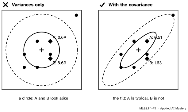
ML02.9.1-F5
Wrong beside right. Without the covariance, \(A\) and \(B\) look equally typical of class 0. With it, \(A\) is well inside the cloud and \(B\) is outside its central ellipse.
“The variances describe the cloud; the covariance is a detail.”
The variances say how wide the cloud is along the two axes. Only the covariance says whether it leans. For class 0 both variances are \({17/9}\), which on their own describe a circle, while the true cloud is a cigar whose long and short axes differ in variance by a factor of more than ten (\({31/9}\) against \({1/3}\)).
“The nearer point to the class mean is the more typical one.”
Only if the cloud is round and equally wide in every direction. Distances must be measured in the cloud’s own units, which differ by direction: that is the Mahalanobis distance. The same rule matters in anomaly detection (ML03.9), where a point can be odd although every one of its features is ordinary.
“np.cov gives the maximum-likelihood covariance.”
By default np.cov divides by \({n - 1}\), the unbiased estimate. The maximum-likelihood estimate, and the one scikit-learn’s discriminant analysis uses, divides by \(n\): pass bias=True. The two differ by the factor \({n/(n - 1)}\), which for a class of six points is 1.2. Note also that np.cov expects the features in rows, so pass X.T.
Check yourself
Recall
1. Which two quantities describe a Gaussian cloud, and what does each control?
Show answer
The mean vector \(\vect{\mu}\) sets where the cloud is centred; the covariance matrix \(\mat{\Sigma}\) sets its width in every direction and its tilt.
2. How are the axes of the contour ellipses related to \(\mat{\Sigma}\)?
Show answer
They point along the eigenvectors of \(\mat{\Sigma}\), and the ellipse \({\Delta = c}\) has semi-axes \(c\sqrt{\lambda_i}\), where the \(\lambda_i\) are the eigenvalues.
3. Write the squared Mahalanobis distance from \(\vect{x}\) to the mean.
4. What do you divide by in the maximum-likelihood covariance of a class, and what does np.cov divide by by default?
Show answer
The number of points in the class, \(n_k\). np.cov divides by \({n_k - 1}\) unless you pass bias=True.
5. Which covariance matrices turn this model into Gaussian naive Bayes?
Show answer
Diagonal ones: with every covariance zero, the density factorises into one bell per feature.
Exercises
1.★ Fit class 1 of the twelve points, (4, 1), (5, 2), (5, 3), (4, 4), (2, 5) and (6, 5): find its mean and maximum-likelihood covariance.
Show solution
The column sums are 26 for \(x_1\), 20 for \(x_2\), 122 for \(x_1^2\), 80 for \(x_2^2\) and 85 for \({x_1x_2}\). The mean is \({(26/6, 20/6) = (13/3, 10/3)}\). The variances are \({122/6 - (13/3)^2 = 14/9}\) and \({80/6 - (10/3)^2 = 20/9}\). The covariance is
and \({\Delta = 2.03}\). The point is 3.77 units away in the plane but only two of the cloud’s units, because it lies along the long axis, the direction in which class 0 spreads most. (Indeed it pulls that axis out: it is one of the six points that define the cloud.)
3.★★★ In the round coordinates \({\vect{z}}\) a two-dimensional Gaussian has density \({\tfrac{1}{2\pi}e^{-(z_1^2 + z_2^2)/2}}\). Show that the probability inside the ellipse \({\Delta = c}\) is \({1 - e^{-c^2/2}}\), and evaluate it for \({c = 1}\) and \({c = 2}\).
Show solution
In the round coordinates the ellipse \({\Delta = c}\) is the disc \({z_1^2 + z_2^2 \le c^2}\). Use polar coordinates \({z_1 = r\cos\theta}\), \({z_2 = r\sin\theta}\), where the area element is \({r\,dr\,d\theta}\):
For \({c = 1}\): \({1 - e^{-0.5} = 0.393}\). For \({c = 2}\): \({1 - e^{-2} = 0.865}\). So the solid ellipses of the anchor figure hold about 39% of each cloud and the dashed ones about 86%.
Summary card
A class is a cloud: a mean, and a covariance that sets its width and its tilt.
Ellipses: axes along the eigenvectors of \(\mat{\Sigma}\), semi-axes \({c\sqrt{\lambda_i}}\).
Fit: class mean, and covariance averaged over \(n_k\) points.
Diagonal \(\mat{\Sigma}\): Gaussian naive Bayes.
Sources and next steps
Sources. Each was opened and checked against this lesson on 15 November 2026.
G. James, D. Witten, T. Hastie and R. Tibshirani, An Introduction to Statistical Learning, 2nd edition (with R, 2021), section 4.4.2: the multivariate Gaussian density, equation (4.23), with mean vector and covariance matrix, and the remark that correlated or unequal-variance predictors give elliptical rather than circular contours (Figure 4.5).
T. Hastie, R. Tibshirani and J. Friedman, The Elements of Statistical Learning, 2nd edition, corrected 12th printing (2017), section 4.3: the class densities as multivariate Gaussians and the estimates of their means and covariances; section 4.3.2 for computing with the eigen-decomposition of each covariance.
scikit-learn, Linear and Quadratic Discriminant Analysis, User Guide section 1.2: the Gaussian class density, the Mahalanobis distance \({(\vect{x} - \vect{\mu}_k)\T \mat{\Sigma}^{-1}(\vect{x} - \vect{\mu}_k)}\), and the statement that diagonal covariances make QDA equivalent to GaussianNB.