When a photo can be tagged sea, people and dog at once, the target is a binary matrix. Binary relevance trains one classifier per label, a classifier chain lets later labels see earlier ones, and subset accuracy, Hamming loss and micro and macro F1 each judge a different thing.
ML02.10.3L2 Intermediate25 minIn review (what this means)
The maths and code on this page are checked by automated tests on every change, but an independent reader has not signed it off yet. Spot a mistake or a confusing step? Tell us.
Store multi-label targets as an n by L binary matrix and tell a multi-label problem from a multi-class one.
Build binary relevance and a classifier chain from a binary learner, and explain what the chain adds.
Compute subset accuracy, Hamming loss and per-label F1 with micro and macro averages by hand.
Choose a metric that matches what a mistake costs, and spot a metric that a trivial model can game.
The question
A photo shows the sea, two people and a dog. A news article is about sport and money. A patient has three diagnoses at once. Every classifier so far picks exactly one class. How do we predict a whole set of labels, and how do we score a prediction that gets two of three tags right?
From the last lesson
1. How many classifiers does one-vs-one train for \(K\) classes, and on which examples?
Show answer
\({K(K - 1)/2}\), one per pair of classes, each trained only on the examples of its two classes.
2. Why does SAMME add \({\ln(K - 1)}\) to the AdaBoost weight?
Show answer
So that the weight stays positive whenever the learner beats random guessing, \({\epsilon_m < (K - 1)/K}\), instead of only when \({\epsilon_m < 1/2}\).
Intuition
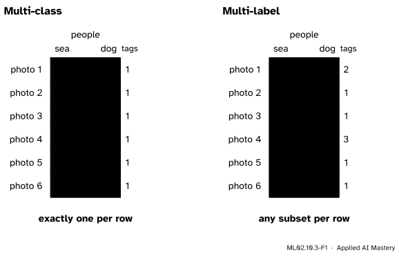
In a multi-label problem each example carries any subset of \(L\) possible labels. Write the targets as a table with one row per example and one column per label, and put a 1 where the label applies. That table is an \(n\) by \(L\) binary matrix \(\mat{Y}\).
ML02.10.3-F1
Six photos and three tags. A multi-class target has exactly one 1 in each row; a multi-label target can have any number, including none.
Multi-class problems are the special case where every row has a single 1. The other direction does not work: a multi-class model must choose one column, so it cannot say “sea and dog”. We need a model with \(L\) yes-or-no outputs.
Build it up
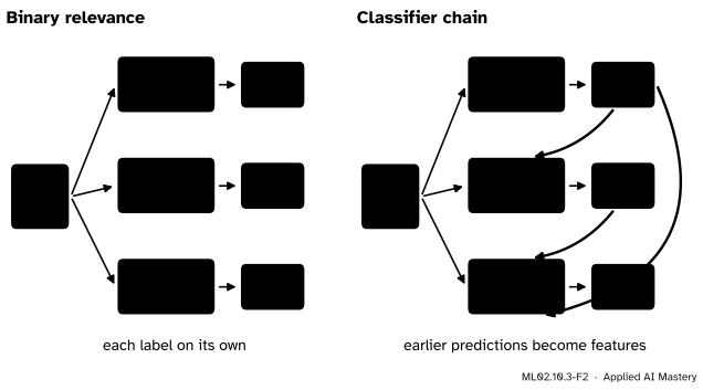
Step 1. One question per label. The simplest model asks \(L\) separate questions: “does this photo show the sea?”, “does it show people?”, “does it show a dog?”. Train one binary classifier per column of \(\mat{Y}\) and stack their answers into a row. This is binary relevance, and scikit-learn’s MultiOutputClassifier does it for any classifier.
Step 2. What binary relevance ignores. Labels go together: beaches come with people more often than with snow; an article tagged “election” is likely tagged “politics”. Binary relevance never sees one label while predicting another.
Step 3. A chain. Put the labels in an order. Classifier 1 predicts label 1 from \(\vect{x}\). Classifier 2 predicts label 2 from \(\vect{x}\) and label 1. Classifier \(j\) sees \(\vect{x}\) and labels 1 to \({j - 1}\). In training the earlier labels are the true ones; at prediction time they are the chain’s own earlier predictions. This is a classifier chain.
ML02.10.3-F2
Binary relevance asks the three questions apart. A chain passes each answer to the classifiers after it, so the dog classifier knows whether the photo was judged a beach photo.
Step 4. Models that do it natively. A decision tree can store a whole row of labels in each leaf: the share of training examples in the leaf that carry each label. Random forests average those shares over trees, so they predict several labels without any wrapper. scikit-learn lists trees, forests and \(k\)-nearest neighbours among the estimators that support multi-label targets.
The formal statement
Why a chain can help. The chain rule of probability writes the joint probability of a label row exactly as a product of conditionals:
A classifier chain fits one factor per classifier. Binary relevance fits \({p(y_j \mid \vect{x})}\) instead, which equals the factor only if the labels are independent once \(\vect{x}\) is known. So the chain aims at the whole row; Read and colleagues tie it to the loss that counts a row as wrong unless every label is right.
Three ways to score. Let \(\hat{\mat{Y}}\) be the predicted matrix.
Subset accuracy\(S\) is the share of rows predicted exactly, every label right. One wrong label spoils a row.
Hamming loss\(\mathrm{HL}\) is the share of cells that are wrong:
Per-label F1 treats each column as its own binary problem (ML01.7.2). The macro average is the mean of the \(L\) scores; the micro average pools the true positives, false positives and false negatives of all columns first. Micro is now not the accuracy, because a multi-label mistake is a false positive or a false negative, not both.
How the first two relate. A row predicted exactly has no wrong cells. A row that is not exact has at least 1 and at most \(L\) wrong cells, out of its \(L\). So
The left end holds when every spoiled row has a single wrong label; the right end when every spoiled row is wrong everywhere.
Worked example
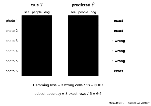
Six photos, three tags, and a model’s predictions.
ML02.10.3-F3
Three cells of eighteen are wrong, one in each of three rows. The other three rows are exact.
Subset accuracy. Rows 1, 2 and 6 are exact: \({S = 3/6 = 0.5}\).
Hamming loss. Three wrong cells out of \({6 \times 3 = 18}\): \({\mathrm{HL} = 3/18 = 0.167}\). Each spoiled row has a single wrong cell, so \({\mathrm{HL} = (1 - S)/L}\), the left end of the inequality.
Per label. Count true positives, false positives and false negatives column by column.
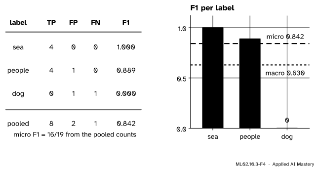
people: \({TP = 4}\), one false positive (photo 5), no false negative: \({F1 = 8/(8 + 1) = 0.889}\).
dog: the one true dog (photo 4) is missed, and photo 3 gets a dog it does not have: \({TP = 0}\), \({FP = 1}\), \({FN = 1}\), so \({F1 = 0}\).
ML02.10.3-F4
The two averages disagree because the rare label, dog, was never right. Macro gives it a third of the say; micro gives it only its share of the counts.
Averages. Macro F1 is the mean of \(1\), \(0.889\) and \(0\), which is \({17/27 = 0.630}\). Micro pools the counts, \({TP = 8}\), \({FP = 2}\), \({FN = 1}\), for \({F1 = 16/19}\)\({= 0.842}\).
Code
The metrics from scratch, checked against scikit-learn, which computes subset accuracy when accuracy_score is given label matrices.
subset accuracy 0.5  Hamming loss 0.167
F1 per label [1.    0.889 0.   ]  macro 0.63  micro 0.842
Now a synthetic problem: make_multilabel_classification draws, for each example, a number of labels from a Poisson distribution with mean n_labels (capped at the number of labels), and then word counts that depend on the labels. Binary relevance and a chain from scratch, both around logistic regression:
from sklearn.base import clonefrom sklearn.datasets import make_multilabel_classificationfrom sklearn.linear_model import LogisticRegressionfrom sklearn.model_selection import train_test_splitX, Y = make_multilabel_classification(n_samples=1000, n_features=20, n_classes=5, n_labels=2, random_state=0)Xtr, Xte, Ytr, Yte = train_test_split(X, Y, test_size=0.3, random_state=0)lr = LogisticRegression(max_iter=2000)L = Y.shape[1]# binary relevance: one classifier per columnP_br = np.column_stack([clone(lr).fit(Xtr, Ytr[:, j]).predict(Xte) for j inrange(L)])# chain: classifier j sees x and the labels before it (true in training, predicted at test)chain = [clone(lr).fit(np.hstack([Xtr, Ytr[:, :j]]), Ytr[:, j]) for j inrange(L)]P_cc = np.zeros_like(Yte)for j, model inenumerate(chain): P_cc[:, j] = model.predict(np.hstack([Xte, P_cc[:, :j]]))print("labels per example:", Y.sum(axis=1).mean(), " examples with none:", int((Y.sum(axis=1) ==0).sum()))for name, P in (("binary relevance", P_br), ("chain", P_cc)):print(f"{name:>16}: subset accuracy {accuracy_score(Yte, P):.3f} Hamming {hamming_loss(Yte, P):.3f}")
wrappers agree: True True
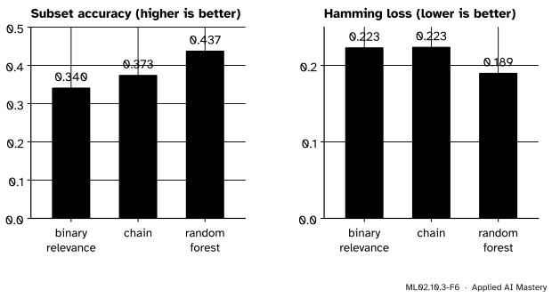
binary relevance: subset 0.340  Hamming 0.223  micro F1 0.678  macro F1 0.680
           chain: subset 0.373  Hamming 0.223  micro F1 0.665  macro F1 0.665
   random forest: subset 0.433  Hamming 0.189  micro F1 0.706  macro F1 0.706
ML02.10.3-F6
On 300 test examples, the chain gets more whole rows right than binary relevance, with the same share of wrong cells; the forest does best on both.
The chain gains on subset accuracy, the metric it aims at, and gains nothing on Hamming loss, which judges labels one at a time; its micro F1 is even a little lower (0.665 against 0.678). Where does the gain come from? The test set has 55 examples with no label at all. The chain predicts an empty row 54 times and gets 33 of those 55 exactly right; binary relevance gets 23. On the other 245 rows both get 79 exactly right. The forest’s numbers depend on its random seed; with logistic regression the first two are fixed by the data.
Explore
This module’s interactive, the reduction explorer in lesson ML02.10.2, shows one-vs-rest by signs. Read its “no class” and “two classes” regions as a multi-label answer: there, binary relevance would honestly predict the empty set or two labels.
Pitfalls
ML02.10.3-F5
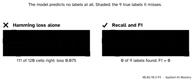
Wrong beside right. With 20 possible labels and about 1.5 per example, a model that predicts nothing is right on most cells. Recall and F1 count only the labels that exist, and show it found none.
“A Hamming loss of 0.075 means the model is good.”
On sparse label sets almost every cell is a 0, so the empty prediction scores well. Always compare with the model that predicts nothing, whose Hamming loss is the share of 1s in \(\mat{Y}\), and report recall or F1 next to it.
“Turn each set of labels into one class and use a multi-class model.”
That is called the label powerset, and it works for a few labels with few combinations. But \(L\) labels have \(2^L\) possible rows: \({2^{20}}\) is over a million classes, most never seen in training, and the model can never predict a combination it has not seen.
“The order of a chain does not matter.”
It does: the first label is predicted from \(\vect{x}\) alone, and an early mistake is passed down the chain. scikit-learn’s ClassifierChain takes order="random", and the User Guide notes that many randomly ordered chains are typically fitted and their predictions averaged.
Check yourself
Recall
1. How are the targets of a multi-label problem stored, and how does a multi-class target look in that form?
Show answer
As an \(n\) by \(L\) binary matrix with a 1 where a label applies. A multi-class target is the special case with exactly one 1 in every row.
2. What does binary relevance ignore?
Show answer
How the labels go together: each label’s classifier never sees the other labels.
3. In a classifier chain, what does classifier \(j\) see during training and at prediction time?
Show answer
The input \(\vect{x}\) and labels 1 to \({j - 1}\): the true labels in training, the chain’s own predictions at prediction time.
4. Define subset accuracy and Hamming loss.
Show answer
Subset accuracy is the share of rows predicted exactly right. Hamming loss is the share of the \(nL\) cells predicted wrong.
5. Why is micro F1 not equal to the accuracy in a multi-label problem?
Show answer
A wrong cell is either a false positive or a false negative, not both, so the pooled false positives and false negatives need not be equal, and micro precision and recall differ.
Exercises
1.★ Three examples, four labels. True rows \({1100}\), \({0011}\), \({1000}\); predicted rows \({1100}\), \({0010}\), \({1001}\). Compute the subset accuracy and the Hamming loss.
Show solution
Row 1 is exact; row 2 misses its last label; row 3 adds a last label. \({S = 1/3}\). Two wrong cells out of 12: \({\mathrm{HL} = 2/12 = 0.167}\).
2.★★ For the exercise above, compute the per-label F1 scores, the macro F1 and the micro F1.
3.★★★ Prove that \({\mathrm{HL} \le 1 - S}\) and \({\mathrm{HL} \ge (1 - S)/L}\), and give a small example where each end is reached.
Show solution
A row counted in \(S\) has no wrong cells. Each of the other \({n(1 - S)}\) rows has between 1 and \(L\) wrong cells. So the number of wrong cells lies between \({n(1 - S)}\) and \({nL(1 - S)}\). Dividing by \(nL\) gives \({(1 - S)/L \le \mathrm{HL} \le 1 - S}\). The worked example reaches the lower end: three spoiled rows, one wrong cell each, \({\mathrm{HL} = 3/18 = (1 - 0.5)/3}\). Predicting the exact complement of every row reaches the upper end: \({S = 0}\) and every cell is wrong, \({\mathrm{HL} = 1}\).
Summary card
Several labels per example: an \(n\) by \(L\) matrix, \(L\) questions, and metrics that count different things.
ML02.10.3-F1
One per row, or any subset.
Binary relevance. One classifier per label, ignoring how labels go together.
Classifier chain. Classifier \(j\) sees \(\vect{x}\) and labels 1 to \({j - 1}\); it targets whole rows.
Subset accuracy. Share of rows exactly right. Hamming loss. Share of cells wrong.
Bounds.\({(1 - S)/L \le \mathrm{HL} \le 1 - S}\).
F1. Per label; macro averages the labels, micro pools the counts.
Sources and next steps
Sources. Each was opened and checked against this lesson on 15 November 2026.
Jesse Read, Bernhard Pfahringer, Geoff Holmes and Eibe Frank, Classifier Chains: A Review and Perspectives, Journal of Artificial Intelligence Research 70 (2021). Section 1: the label vector, binary relevance as independent binary classifiers, and the chain in which each prediction becomes a feature of the classifiers after it. Section 2.1: chains as models of the joint probability, aimed at the 0/1 loss on whole rows; Section 2.2: chains often help under Hamming loss too, but with strong base learners that gain can in theory shrink to nothing, and in practice it varies with the data.
scikit-learn 1.9 User Guide, Section 1.12.2: the label matrix, MultiOutputClassifier fitting one classifier per target, ClassifierChain fitting each model on the features plus earlier labels and passing predictions on, the advice to average several randomly ordered chains, and the list of estimators that support multi-label targets. Section 3.4.4: subset accuracy (3.4.4.2), the Hamming loss formula (3.4.4.8) and the micro and macro averages (3.4.4.1).
scikit-learn 1.9, make_multilabel_classification: the number of labels per example drawn from a Poisson distribution with mean n_labels and bounded by n_classes, and allow_unlabeled=True by default.
Next.ML02.10.4 Ordinal targets returns to one label per example, but with classes that come in an order.