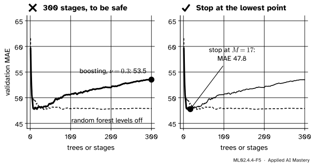
Boosting fits its training data ever more closely, so it can overfit. Three settings control it: a learning rate that takes small steps, a tree depth that limits interactions, and a number of stages chosen by early stopping. Measured on load_diabetes with the folds of the ML01.10 project.
ML02.4.4L2 Intermediate25 minIn review (what this means)
The maths and code on this page are checked by automated tests on every change, but an independent reader has not signed it off yet. Spot a mistake or a confusing step? Tell us.
Explain how the learning rate trades fewer large steps for more small ones, and compute the effect of shrinkage on the first stage exactly.
Relate the depth of the trees to the order of feature interactions a boosted model can represent.
Describe stochastic gradient boosting and what subsample does.
Choose the number of stages by early stopping, from scratch with staged_predict and with n_iter_no_change.
The question
Run gradient boosting on the diabetes data of the ML01.10 project with a learning rate of \(1\) and depth-2 trees. The validation error is lowest after four stages; by stage 300 it is worse than after one. A random forest given 300 trees just levels off. Why does boosting overfit when a forest does not, and which settings decide how well a boosted model does on data it has not seen?
From the last lesson
1. In gradient boosting for classification, what are the trees fitted to?
Show answer
The pseudo-residuals \({y_i - p_i}\): the label minus the current predicted probability, the negative gradient of the log loss with respect to the score.
2. What is the Newton leaf value, in terms of the leaf sums \(G\) and \(H\)?
Show answer
\({\gamma = -G/H}\), with \({G = \sum (p_i - y_i)}\) and \({H = \sum p_i(1 - p_i)}\).
Intuition
Every stage of boosting fits the residuals of the stages before it, so the training error keeps falling (lesson ML02.4.1). Early stages capture the broad shape of the data. Later ones chase smaller and smaller patterns, and after a point those patterns are noise. That is overfitting, and it is why boosting needs a brake that a forest of independent, averaged trees does not.
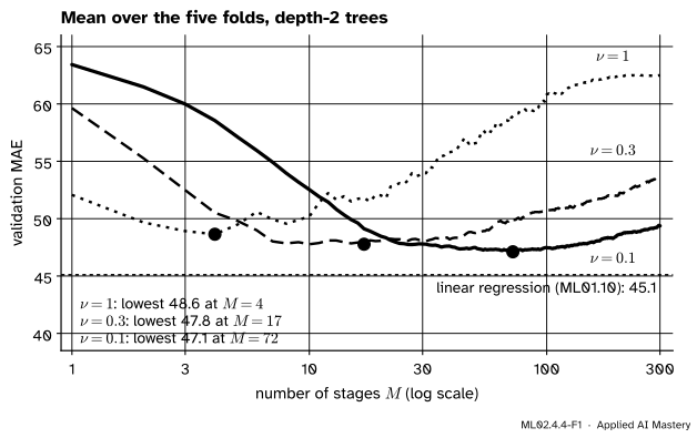
The main brake is the learning rate\({\cparam{\nu}}\): add only a fraction of each tree. The figure shows the validation error of the diabetes model, averaged over the five folds of ML01.10, for three learning rates.
ML02.4.4-F1
Validation error against the number of stages for three learning rates. A smaller \(\cparam{\nu}\) needs more stages to reach its lowest point, reaches a lower one, and climbs back more slowly.
Three things are visible. Each curve has a lowest point and then rises: boosting overfits. A smaller \(\cparam{\nu}\) reaches a lower minimum. And it gets there later, so it costs more trees. The recipe that follows from this, set \(\cparam{\nu}\) small and stop at the lowest point, is the standard way to run gradient boosting.
Build it up
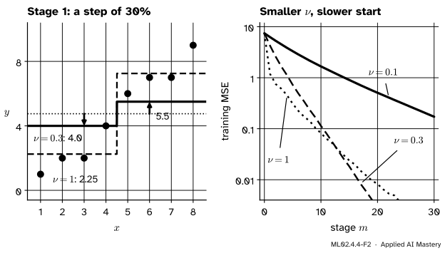
Step 1. Shrinkage. The update becomes \({F_m = F_{m-1} + \cparam{\nu}\, h_m}\) with \({0 < \cparam{\nu} \le 1}\). On the eight points, the first stump with \({\cparam{\nu} = 0.3}\) moves the predictions only from \(4.75\) to \(4.0\) and \(5.5\) instead of to \(2.25\) and \(7.25\). The residuals stay large, and later stumps get to spend them on other splits.
ML02.4.4-F2
Left: with \({\cparam{\nu} = 0.3}\) the first stump moves each prediction 30 percent of the way. Right: the training error starts to fall more slowly for smaller \(\cparam{\nu}\), and \({\cparam{\nu} = 0.1}\) is still far behind at stage 30. Full steps are not always the fastest route down, though: from stage 13 on, \({\cparam{\nu} = 0.3}\) is below \({\cparam{\nu} = 1}\).
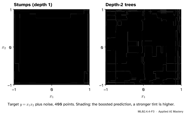
Step 2. Tree depth. A stump splits on one feature, so a sum of stumps can add an effect of \(x_1\) to an effect of \(x_2\) but cannot make the effect of \(x_2\) depend on \(x_1\). A depth-2 tree splits on one feature and then, inside each half, possibly on another, which is a two-feature interaction. The figure boosts the target \({y = x_1 x_2}\), where the sign of the effect of \(x_2\) flips with the sign of \(x_1\).
ML02.4.4-F3
Boosting on \({y = x_1 x_2}\). Stumps find nothing, because averaged over \(x_2\) the effect of \(x_1\) is zero, and the other way round. Depth-2 trees recover the four quadrants.
Step 3. Subsampling. Fit each tree on a random fraction of the training rows, drawn without replacement afresh at every stage. This is stochastic gradient boosting. It makes each tree cheaper and a little noisier, and, like bagging, the noise can help generalisation.
Step 4. Early stopping. Hold out a validation set, record its error after every stage, and keep the number of stages \(M\) where it is lowest.
The formal statement
Shrinkage on the first stage, exactly. Let a stump with leaf means \(h(x_i)\) be fitted to residuals \(r_i\). With shrinkage, the new residuals are \({r_i - \cparam{\nu} h(x_i)}\). Split each one as
Within a leaf, \(h_i\) is a constant, the mean of the \(r_i\), so the deviations \({r_i - h_i}\) add up to zero there. Squaring and summing, the cross term \({2(1 - \cparam{\nu}) \sum (r_i - h_i) h_i}\) vanishes leaf by leaf, leaving
The first sum is what the full stump leaves; the second is the part of the fit that shrinkage holds back. On the eight points, the full stump leaves \(9.5\) and \({\sum h_i^2 = 8 \times 2.5^2 = 50}\), so \({\text{SSE}(\cparam{\nu}) = 9.5 + 50(1 - \cparam{\nu})^2}\): \(9.5\), \(22\), \(34\) and \(50\) for \({\cparam{\nu} = 1, 0.5, 0.3, 0.1}\), or MSEs \(1.1875\), \(2.75\), \(4.25\) and \(6.25\).
Depth and interactions. A tree of depth \(D\) reaches each leaf through at most \(D\) splits, so the indicator of each leaf’s region depends on at most \(D\) features. The tree as a whole may use more features (a depth-2 tree can split on \(x_1\), then on \(x_2\) in one half and \(x_3\) in the other), but it is a sum of leaf value times leaf indicator, so it is a sum of functions of at most \(D\) features each, and so is a sum of such trees. For stumps, \({D = 1}\), collect the stumps that split on feature \(j\) into one function \(f_j\); with \(d\) features,
an additive model with main effects only. ESL (Section 10.11) counts leaves instead: a tree with \(J\) leaves allows interactions of order at most \({J - 1}\), and a stump has \({J = 2}\).
Early stopping. With validation error \(E_m\) after stage \(m\), the early-stopping choice is \({M^* = \argmin_m E_m}\). scikit-learn’s rule with n_iter_no_change\(= k\) stops training as soon as the validation loss has failed to improve by at least tol for \(k\) stages in a row, on a validation_fraction of the training rows held out automatically.
Go deeper: why small steps generalise better
There is no single proof, but two views help. First, shrinkage makes boosting behave like a regularised fit: ESL Section 16.2.1 connects forward stagewise fitting with tiny steps to the lasso’s L1 penalty, so a small \(\cparam{\nu}\) with \(M\) stopped early is like a lasso with a moderate penalty. Second, a large step commits fully to the first tree’s splits, which were chosen greedily on noisy data. Small steps leave most of each residual for later trees, so many different splits share the fit and no single greedy choice dominates. ESL Section 10.12.1 reports the empirical finding of Friedman (2001) that smaller \(\cparam{\nu}\) gives better test error, at the price of more stages.
Worked example
Two stages on the eight points with \({\cparam{\nu} = 0.5}\).
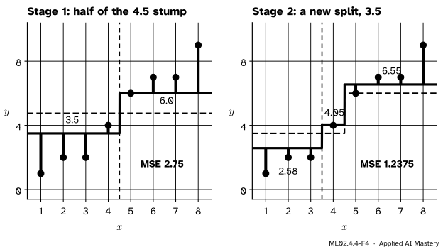
Stage 1. The stump is the same as before: split at \(4.5\), leaves \(-2.5\) and \(2.5\). Half of it moves the predictions to \({4.75 - 1.25 = 3.5}\) and \({4.75 + 1.25 = 6.0}\). The residuals are (−2.5, −1.5, −1.5, 0.5, 0, 1, 1, 3), and their squares add to
Stage 2. Half a step was taken at \(4.5\), so that split still explains something (squared error \(9.5\)), but the split at \(3.5\) now does better. Its left leaf holds \((-2.5, -1.5, -1.5)\), mean \({-11/6 \approx -1.833}\); its right leaf holds (0.5, 0, 1, 1, 3), mean \(1.1\). The squared deviations add up to \({2/3}\) on the left and \(5.2\) on the right, \(5.87\) in all, against \(9.5\) at \(4.5\). Half of this stump is added:
The squared residuals add up to \(9.9\), an MSE of \({9.9/8 = 1.2375}\).
ML02.4.4-F4
Two half steps. Because stage 1 left half of the \(4.5\) jump unfitted, stage 2 is free to choose a different split, and the staircase gains a level at \(x = 4\).
With \({\cparam{\nu} = 1}\) the training MSE after two stages was \(0.75\); here it is \(1.2375\). Smaller steps fit the training data more slowly, and that is the point: what matters is the validation error, and there the slow learner wins.
Code
First the shrinkage formula, checked against a direct computation on the eight points.
import numpy as npx = np.arange(1.0, 9.0)y = np.array([1, 2, 2, 4, 6, 7, 7, 9], dtype=float)h = np.where(x <=4.5, -2.5, 2.5) # the first stumpfor nu in (1.0, 0.5, 0.3, 0.1): direct = np.sum((y - (y.mean() + nu * h)) **2)print(f"nu = {nu}: SSE {direct:.2f}, formula {9.5+50* (1- nu) **2:.2f}")
nu = 1.0: SSE 9.50, formula 9.50
nu = 0.5: SSE 22.00, formula 22.00
nu = 0.3: SSE 34.00, formula 34.00
nu = 0.1: SSE 50.00, formula 50.00
Now load_diabetes, with the working rows and the five folds of ML01.10. staged_predict gives the validation predictions after every stage from a single fit, so one fit per fold traces a whole curve.
from sklearn.datasets import load_diabetesfrom sklearn.ensemble import GradientBoostingRegressorfrom sklearn.model_selection import KFold, train_test_splitdata = load_diabetes(scaled=False)X_work, X_test, y_work, y_test = train_test_split(data.data, data.target, test_size=89, random_state=10)folds =list(KFold(n_splits=5).split(X_work))def curve(**settings):"""Validation MAE after each stage, averaged over the five folds.""" per_fold = []for train, valid in folds: model = GradientBoostingRegressor(max_depth=2, n_estimators=300, random_state=0, **settings) model.fit(X_work[train], y_work[train]) per_fold.append([np.mean(np.abs(y_work[valid] - p)) for p in model.staged_predict(X_work[valid])])return np.mean(per_fold, axis=0)curves = {nu: curve(learning_rate=nu) for nu in (1.0, 0.3, 0.1)}for nu, c in curves.items():print(f"nu = {nu}: lowest {c.min():.1f} at M = {c.argmin() +1}, after 300 stages {c[-1]:.1f}")stochastic = curve(learning_rate=0.1, subsample=0.5)print(f"subsample 0.5: lowest {stochastic.min():.1f} at M = {stochastic.argmin() +1}")
nu = 1.0: lowest 48.6 at M = 4, after 300 stages 62.5
nu = 0.3: lowest 47.8 at M = 17, after 300 stages 53.5
nu = 0.1: lowest 47.1 at M = 72, after 300 stages 49.4
subsample 0.5: lowest 46.8 at M = 47
The ordering is the one of the anchor figure. For comparison, the linear regression of ML01.10 scored \(45.1\) on the same folds: on this small, nearly linear dataset, boosting does not win. Subsampling half the rows lowers the best error a little, from \(47.1\) to \(46.8\).
Early stopping in the library: n_iter_no_change holds out validation_fraction of the rows and stops when the validation loss has not improved for that many stages.
Stumps do worse than predicting zero: with no main effects to find, they fit noise. Depth-2 trees cut the error several times over.
Explore
The residual stepper in lesson ML02.4.1 has a learning-rate slider and a validation curve. Choose the noisy sine and depth-2 trees, then compare \({\cparam{\nu} = 1}\) with \({\cparam{\nu} = 0.1}\): note the stage where each validation curve bottoms out, and how low it gets.
Pitfalls
ML02.4.4-F5
Wrong beside right. A forest’s error levels off as trees are added; boosting’s error turns back up. Running boosting for many stages “to be safe” gives \(53.5\); stopping at stage 17 gives \(47.8\).
“More trees can only help, as in a random forest.”
A forest averages independent trees, so extra trees only reduce variance. Boosting adds trees that fit the remaining residuals, so extra trees keep fitting, noise included. The number of stages is a setting to tune, by early stopping or cross-validation.
“A smaller learning rate is always better.”
It usually generalises better, but each halving of \(\cparam{\nu}\) roughly doubles the number of stages, and the gain shrinks: here \({\cparam{\nu} = 0.3}\) to \(0.1\) improved the best error by only \(0.7\) while needing four times as many trees. Pick \(\cparam{\nu}\) as small as the time budget allows and let early stopping pick \(M\).
“Choose the number of stages on the test set.”
Early stopping is tuning. Use a validation set or the cross-validation folds, as here, and keep the test rows of ML01.10 locked until the end, or the test score will flatter the model.
Check yourself
Recall
1. What does the learning rate \(\cparam{\nu}\) do to each stage of boosting?
Show answer
It scales each tree before it is added, \({F_m = F_{m-1} + \cparam{\nu}\, h_m}\), so each stage takes only a fraction of the step the tree suggests.
2. Why can a sum of stumps not represent an interaction between two features?
Show answer
Each stump depends on one feature, so the sum is an additive model \({\sum_j f_j(x_j)}\): the effect of \(x_2\) is the same whatever \(x_1\) is.
3. What is stochastic gradient boosting?
Show answer
Gradient boosting in which each tree is fitted on a random fraction of the training rows, drawn without replacement at every stage (subsample < 1 in scikit-learn).
4. On the eight points, what is the training MSE after one stage with \({\cparam{\nu} = 0.3}\)?
Show answer
\({(9.5 + 50 \times 0.7^2)/8 = 34/8 = 4.25}\).
5. How does early stopping choose the number of stages?
Show answer
It tracks a validation error after every stage and keeps the stage where it is lowest; scikit-learn’s n_iter_no_change stops once the validation loss has not improved for that many stages.
Exercises
1.★ Using the shrinkage formula, find the learning rate at which the first stump on the eight points leaves a training MSE of \(2\).
Show solution
An MSE of \(2\) is an SSE of \(16\). Then \({9.5 + 50(1 - \cparam{\nu})^2 = 16}\), so \({(1 - \cparam{\nu})^2 = 0.13}\) and \({1 - \cparam{\nu} = \sqrt{0.13} \approx 0.361}\), giving \({\cparam{\nu} \approx 0.639}\).
2.★★ A boosted model uses stumps on three features. Show that its prediction can be written as \({F_0 + f_1(x_1) + f_2(x_2) + f_3(x_3)}\), and say how many levels \(f_1\) can have if \(20\) of the \(M = 50\) stumps split on \(x_1\).
Show solution
Each stump is \({\cparam{\nu}\, h_m(x_{j_m})}\) for the one feature \(j_m\) it splits on. Grouping the stumps by feature, \({f_j(x_j) = \cparam{\nu} \sum_{m:\, j_m = j} h_m(x_j)}\), and the model is \(F_0\) plus the three sums. The \(20\) stumps on \(x_1\) have at most \(20\) distinct thresholds, so \(f_1\) is a step function with at most \(20\) jumps and so at most \(21\) levels (fewer if thresholds repeat).
3.★★★ Generalise the shrinkage formula: show that for any stage and any regression tree with leaf means, the SSE after the shrunken update is the SSE of the full update plus \({(1 - \cparam{\nu})^2 \sum h_i^2}\), and deduce the fraction of the full stage’s improvement that a shrunken stage achieves.
Show solution
The derivation in the formal statement used only that \(h_i\) is constant within each leaf and equal to the mean of the \(r_i\) there, which holds for any regression tree with mean leaves at any stage. So \({\text{SSE}(\cparam{\nu}) = \text{SSE}(1) + (1 - \cparam{\nu})^2 \sum h_i^2}\). With \({\cparam{\nu} = 0}\) nothing changes, so \({\text{SSE}(0) = \sum r_i^2 = \text{SSE}(1) + \sum h_i^2}\): the full stage improves the SSE by \({\sum h_i^2}\). The shrunken stage improves it by \({\sum h_i^2 - (1 - \cparam{\nu})^2 \sum h_i^2}\), a fraction \({1 - (1 - \cparam{\nu})^2 = \cparam{\nu}(2 - \cparam{\nu})}\) of the full improvement. With \({\cparam{\nu} = 0.1}\), a stage achieves \(19\) percent of what the full stage would.
Summary card
Small steps, shallow trees, and stop at the lowest validation error.
ML02.4.4-F1
Lower and later as \(\cparam{\nu}\) shrinks.
Shrinkage.\({F_m = F_{m-1} + \cparam{\nu}\, h_m}\). A shrunken stage keeps a fraction \({\cparam{\nu}(2 - \cparam{\nu})}\) of the full stage’s gain.
Depth. Depth-\(D\) trees allow interactions of up to \(D\) features; stumps give an additive model.
Subsampling. Each tree on a random fraction of rows (subsample).
Early stopping.\({M^* = \argmin_m E_m}\); n_iter_no_change, validation_fraction.
Diabetes. Best MAE \(48.6\), \(47.8\), \(47.1\) for \({\cparam{\nu} = 1, 0.3, 0.1}\).
Sources and next steps
Sources. Each was opened and checked against this lesson on 15 November 2026.
Trevor Hastie, Robert Tibshirani and Jerome Friedman, The Elements of Statistical Learning, 2nd edition, 12th printing. Section 10.11: no interaction effects of level greater than \({J - 1}\) are possible with \(J\)-leaf trees, and stumps give main effects only. Section 10.12: each iteration usually reduces the training risk, and the number of iterations is estimated on a validation sample, as in early stopping. Section 10.12.1 gives the shrunken update (10.41) and reports that smaller \(\nu\) favours better test error with more iterations (Friedman, 2001). Section 10.12.2 describes stochastic gradient boosting, sampling a fraction of the rows without replacement, typically one half. Section 16.2.1, to which Section 10.12.1 points, links shrunken forward stagewise fitting to the lasso.
Gareth James, Daniela Witten, Trevor Hastie and Robert Tibshirani, An Introduction to Statistical Learning, 2nd edition, Section 8.2.3. Boosting’s three tuning parameters: the number of trees, which “can overfit if B is too large”; the shrinkage \(\lambda\); and the number of splits \(d\), the interaction depth, with stumps giving an additive model.
scikit-learn developers, GradientBoostingRegressor and User Guide 1.11.1.2, version 1.9.1. The parameters learning_rate, subsample (“Stochastic Gradient Boosting”), max_depth, n_iter_no_change, validation_fraction and tol, the attribute n_estimators_, and staged_predict for monitoring the error after each stage.
Next. Module ML02.5, XGBoost, LightGBM and CatBoost, adds a penalty to the leaf values, scores splits with the Newton quadratic of lesson ML02.4.3, and makes the whole loop fast.