Covariance is symmetric and linear in each slot. Derive those rules, then the variance of any sum, Var(X) + Var(Y) + 2 Cov(X, Y), find the course’s covariance again from the flip the two counts share, and see why an ensemble wants errors that do not move together.
M06.10.2L1 Core25 minIn review (what this means)
The maths and code on this page are checked by automated tests on every change, but an independent reader has not signed it off yet. Spot a mistake or a confusing step? Tell us.
Derive Cov(aX + b, Y) = a Cov(X, Y) and Cov(X + W, Y) = Cov(X, Y) + Cov(W, Y), and use them to expand the covariance of sums.
Derive Var(X + Y) = Var(X) + Var(Y) + 2 Cov(X, Y), with the independent case of M06.7.3 as the special case Cov = 0.
Find the covariance of the course’s table again as the variance of the shared flip, and check Var(X + Y) = 3/2 against the PMF of X + Y.
Write the 2 by 2 covariance matrix of a pair, and compute the variance of the average of two predictors as (σ² + Cov)/2.
The question
Two models predict house prices, and each is off by an error with variance 4. Average their predictions. If the two errors were independent, the variance of the average would be 2, half of either one. But two models trained on the same data tend to make the same mistakes. How much does averaging help then, and what number decides it?
\({\operatorname{Var}(X)}\): with \({Y = X}\) every rectangle is a square.
Intuition
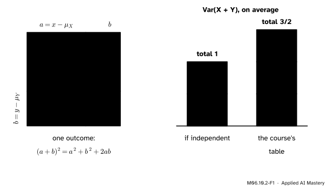
Take one outcome. Call its two deviations \({a = x - \mu_X}\) and \({b = y - \mu_Y}\). The deviation of the sum \({X + Y}\) from its mean \({\mu_X + \mu_Y}\) is then \({a + b}\), and its square is a square of side \({a + b}\). Cut that square along the two sides and it falls into four pieces: a square \(a^2\), a square \(b^2\), and two rectangles \(ab\).
M06.10.2-F1
Left: for one outcome, the square on the deviation of the sum is two squares and two rectangles. Right: averaged over the course’s table, the squares give the two variances and the rectangles give twice the covariance, \({1/2 + 1/2 + 1/2 = 3/2}\).
Average each piece over all outcomes. The squares average to \({\operatorname{Var}(X)}\) and \({\operatorname{Var}(Y)}\). The rectangles are the rectangles of M06.10.1, and they average to the covariance, twice. So the spread of a sum is the two spreads plus twice the covariance. When the variables move together the sum spreads more; when they move apart it spreads less.
Build it up
Step 1. Order does not matter. The rectangle of the point \({(x, y)}\) has the same area as the rectangle of \({(y, x)}\), so \({\operatorname{Cov}(X, Y) = \operatorname{Cov}(Y, X)}\).
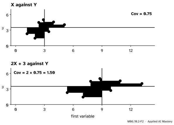
Step 2. A shift changes nothing. Add 3 to every value of \(X\). Every point moves 3 to the right, and so does the mean of \(X\). No deviation changes, so no rectangle changes.
Step 3. A stretch scales the rectangles. Double every value of \(X\). Each horizontal deviation doubles, so every rectangle is twice as wide and the covariance doubles. Multiply by \(-1\) instead and every rectangle flips sign.
M06.10.2-F2
\({2X + 3}\) against \(Y\). The shift by 3 moves the points and their mean together, so it changes no rectangle; the stretch by 2 doubles every width, so it doubles the covariance.
Step 4. A sum in one slot splits. The deviation of \({X + W}\) is the deviation of \(X\) plus the deviation of \(W\). A rectangle whose width is a sum of two widths is two rectangles side by side.
The formal statement
NoteRules of covariance
For random variables \(X\), \(W\), \(Y\) and numbers \(a\), \(b\):
Sum. The mean of \({X + W}\) is \({\mu_X + \mu_W}\), so its deviation is \({(X - \mu_X) + (W - \mu_W)}\). Multiply by \({Y - \mu_Y}\) and use linearity:
Together these rules say that covariance is linear in each slot, so the covariance of two sums expands like a product of two brackets: every piece of the first with every piece of the second.
The variance of a sum. A variance is a covariance with itself, so expand both slots:
For independent \(X\) and \(Y\), \({\E[XY] = \E[X]\,\E[Y]}\) (M06.7.2), so the covariance is 0 and the rule of M06.7.3 comes back: variances add. The same expansion with \({aX + bY}\) gives the general form
and with \({a = 1}\), \({b = -1}\), the difference: \({\operatorname{Var}(X - Y)}\)\({= \operatorname{Var}(X) + \operatorname{Var}(Y)}\)\({- 2\operatorname{Cov}(X, Y)}\).
The covariance matrix, a first look. The three numbers in that formula fit in a 2 by 2 table, the covariance matrix of the pair: variances on the diagonal, the covariance off it. For the course’s table,
It is symmetric because covariance is. The variance of any combination \({aX + bY}\) is read off it: \(a^2\) times the top left, \(b^2\) times the bottom right, \(2ab\) times the corner. Principal component analysis (M03.6) and the multivariate Gaussian (M07.3) are built on this matrix.
Go deeper: the same formula as a matrix product
Put the weights in a column \({\vect{w} = (a, b)}\). Then the variance of \({aX + bY}\) is \({\vect{w}\T \mat{\Sigma}\, \vect{w}}\). Multiplying out,
which is the formula above because \({\Sigma_{12} = \Sigma_{21}}\). Since a variance is never negative, \({\vect{w}\T \mat{\Sigma}\, \vect{w} \ge 0}\) for every \(\vect{w}\): a covariance matrix is always positive semidefinite, the property M03.4 studies.
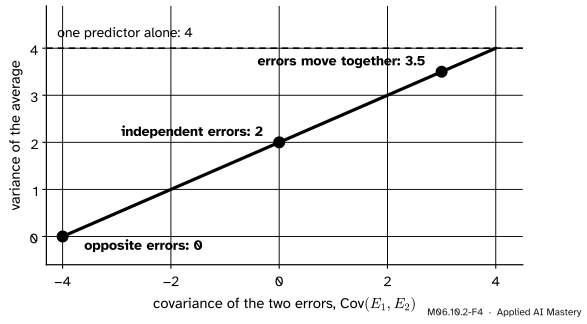
Averaging two predictors. Let \({E_1}\) and \({E_2}\) be the errors of two predictors, each with variance \({\sigma^2}\) and covariance \(C\). The averaged prediction has error \({(E_1 + E_2)/2}\), so by the rule with \({a = b = 1/2}\):
Two predictors whose errors each have variance 4. The variance of their average is \({(4 + C)/2}\): half of 4 when the errors are independent, 3.5 when their covariance is 3, and no gain at all when it reaches 4.
With \({\sigma^2 = 4}\): independent errors give 2; errors with covariance 3 give 3.5, barely better than one predictor. This is why an ensemble (ML02.2) is built from members that err differently: different data, different features, different kinds of model. However many members are added, the variance of the average never falls below the covariance they share (exercise 3).
Worked example
The course’s covariance, found again. Let \({H_1, H_2, H_3}\) be 1 for a head and 0 for a tail on the three flips. Each has variance \({\tfrac12 \cdot \tfrac12 = \tfrac14}\) (a Bernoulli variable, M06.7.3). The flips are independent, so for \({i \ne j}\), \({\E[H_i H_j] = \E[H_i]\,\E[H_j]}\) and \({\operatorname{Cov}(H_i, H_j) = 0}\).
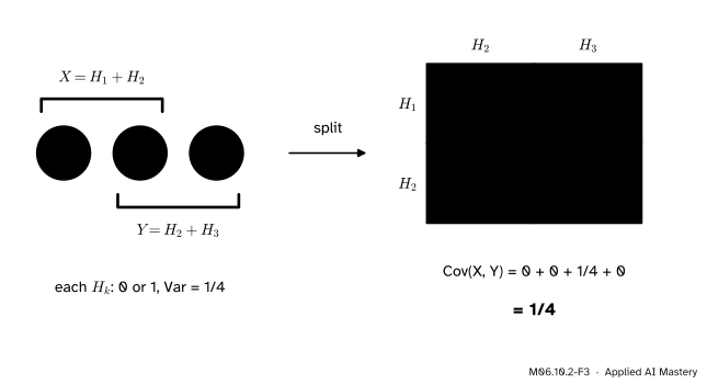
Now \({X = H_1 + H_2}\) and \({Y = H_2 + H_3}\). Expand both slots, every piece with every piece:
Cov(X, Y) by the rules. Each count is split into flips, and the covariance into one cell per pair of flips. Only the shared flip, \({H_2}\) with itself, contributes: its variance, \({1/4}\).
The covariance of the two counts is the variance of the one flip they share, the same \({1/4}\) that the table gave in M06.10.1, now with a reason.
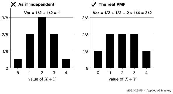
Check it directly. \({X + Y = H_1 + 2H_2 + H_3}\) takes the values 0 to 4 with probabilities \({\tfrac18, \tfrac28, \tfrac28, \tfrac28, \tfrac18}\) (count the eight outcomes). Its mean is 2, and
The variance of the difference.\({\operatorname{Var}(X - Y)}\)\({= \tfrac12 + \tfrac12 - 2 \cdot \tfrac14}\)\({= \tfrac12}\). Check: \({X - Y = H_1 - H_3}\), the shared flip cancels, and two independent flips give \({\tfrac14 + \tfrac14 = \tfrac12}\).
Code
From scratch, with every variable a function of the eight equally likely outcomes, so that each rule is checked exactly.
Now the covariance matrix from simulated flips, and the two predictors. Their errors are built as a shared part \(S\) with variance 3 plus a private part with variance 1, so each error has variance 4 and the two have covariance 3.
covariance matrix:
 [[0.5   0.25 ]
 [0.25  0.499]]
each error: 3.99 3.98   covariance: 2.99
variance of the average: 3.49   formula (4 + 3)/2 = 3.5
Explore
The correlation explorer of M06.10.3 shows the rule for a stretch at work: switch the heights from metres to centimetres, which multiplies them by 100, and watch the covariance grow by exactly that factor.
Pitfalls
M06.10.2-F5
Wrong beside right. Adding the variances treats the two counts as independent and predicts the peaked PMF on the left. The real sum spreads further, because both counts rise with the shared flip.
“Variances add.”
Only when the covariance is 0, for example for independent variables. For the course’s table \({\operatorname{Var}(X) + \operatorname{Var}(Y) = 1}\), but \({\operatorname{Var}(X + Y) = 3/2}\). In a sum of measurements that share a source of error, such as readings from one badly calibrated instrument, the shared part does not average away.
“Cov(2X, 2Y) = 2 Cov(X, Y).”
The rule applies in each slot: \({\operatorname{Cov}(2X, 2Y)}\)\({= 2 \cdot 2 \operatorname{Cov}(X, Y)}\)\({= 4\operatorname{Cov}(X, Y)}\). Doubling both variables doubles both sides of every rectangle, so each area grows four times, just as \({\operatorname{Var}(2X) = 4\operatorname{Var}(X)}\).
“Var(X − Y) = Var(X) − Var(Y).”
The variances still add; only the covariance term changes sign: \({\operatorname{Var}(X - Y)}\)\({= \operatorname{Var}(X) + \operatorname{Var}(Y)}\)\({- 2\operatorname{Cov}(X, Y)}\). For the course’s table that is \({1/2}\), not 0. A positive covariance makes a difference less variable, which is why comparing two models on the same test examples (a paired comparison) gives a steadier verdict than comparing them on separate examples.
Check yourself
Recall
1. What is \({\operatorname{Cov}(aX + b, Y)}\)?
Show answer
\({a\operatorname{Cov}(X, Y)}\). The shift \(b\) cancels from the deviations; the stretch \(a\) scales them.
4. For the course’s table, why is \({\operatorname{Cov}(X, Y) = 1/4}\)?
Show answer
\({X = H_1 + H_2}\) and \({Y = H_2 + H_3}\); expanding, only \({\operatorname{Cov}(H_2, H_2)}\)\({= \operatorname{Var}(H_2) = 1/4}\) survives, because different flips are independent.
5. Two predictors’ errors each have variance \({\sigma^2}\) and covariance \(C\). What is the variance of the error of their average?
2.★★ For the course’s table, find \({\operatorname{Cov}(X, X + Y)}\) and \({\operatorname{Cov}(X + Y, X - Y)}\).
Show solution
\({\operatorname{Cov}(X, X + Y)}\)\({= \operatorname{Var}(X) + \operatorname{Cov}(X, Y)}\)\({= 1/2 + 1/4}\)\({= 3/4}\). For the second, expand both slots:
The sum and the difference of two variables with equal variances always have covariance 0.
3.★★★ An ensemble averages \(n\) predictors. Each error has variance \({\sigma^2}\) and every pair of errors has covariance \(C\). Show that the averaged error has variance \({C + (\sigma^2 - C)/n}\), and evaluate it for \({\sigma^2 = 4}\), \({C = 3}\), \({n = 10}\).
Show solution
Expand the covariance of the sum with itself: \(n\) variances, one for each predictor, and a covariance for each ordered pair \({i \ne j}\), of which there are \({n(n - 1)}\):
For \({\sigma^2 = 4}\), \({C = 3}\), \({n = 10}\): \({3 + 1/10 = 3.1}\). However many members are added, the variance never falls below the shared part \(C\).
Summary card
The variance of a sum is two variances plus twice the covariance.
M06.10.2-F1
Two squares, two rectangles.
\({\operatorname{Cov}(aX + b, Y)}\)\({= a\operatorname{Cov}(X, Y)}\); covariance is linear in each slot.
Covariance matrix: variances on the diagonal, covariances off it.
Average of two predictors: \({(\sigma^2 + C)/2}\).
Sources and next steps
Sources. Each was opened and checked against this lesson on 14 November 2026.
Hossein Pishro-Nik, Covariance and Correlation, Section 5.3.1 of Introduction to Probability, Statistics, and Random Processes: Lemma 5.3 (symmetry, \({\operatorname{Cov}(aX, Y) = a\operatorname{Cov}(X, Y)}\), adding a constant changes nothing, additivity in each argument, and the double-sum form for linear combinations) and Equation 5.21 for \({\operatorname{Var}(aX + bY)}\).
Jeremy Orloff and Jonathan Bloom, Reading 7b: Covariance and Correlation, MIT OpenCourseWare 18.05, Spring 2022. Section 2.1 lists the properties, including \({\operatorname{Var}(X + Y)}\)\({= \operatorname{Var}(X) + \operatorname{Var}(Y)}\)\({+ 2\operatorname{Cov}(X, Y)}\); Example 1 in Section 2.3 redoes the three-flip covariance with \({X = X_1 + X_2}\) and \({Y = X_2 + X_3}\), where only \({\operatorname{Cov}(X_2, X_2) = 1/4}\) survives; Section 4.1 proves the properties.
NumPy, numpy.cov: two 1-D inputs give the 2 by 2 covariance matrix, variances on the diagonal.
Next.M06.10.3 Correlation: covariance without units divides the covariance by the two standard deviations, proves that the result lies between −1 and 1, and finds it inside the best straight line.