Run n independent trials, each a success with chance p, and count the successes. Derive the binomial PMF as a count of sequences times the chance of each, get its mean np and variance np(1 - p) from indicators, and score a classifier on 10 test examples.
M06.8.1L1 Core25 minIn review (what this means)
The maths and code on this page are checked by automated tests on every change, but an independent reader has not signed it off yet. Spot a mistake or a confusing step? Tell us.
State the binomial story and recognise when a count of successes follows it.
Derive the binomial PMF as the number of sequences with k successes times the chance of each one, and show that it sums to 1.
Derive the mean np and the variance np(1 - p) by writing the count as a sum of independent indicators.
Compute binomial probabilities by hand, with math.comb and fractions, by simulation and with scipy.stats.binom.
The question
A classifier is right on 90% of the examples it will ever see. You test it on 10 fresh examples. How likely is a perfect score of 10 out of 10? And how likely is a score of 8 or less, which makes a good model look worse than it is? Every accuracy you read off a small test set is one draw from the distribution this lesson builds.
Intuition
Some random numbers are counts of successes: correct predictions on a test set, heads in a run of flips, users out of 50 who click. They share one story.
Run \(n\) trials. Each trial is a success with the same chance \(p\), whatever the other trials did. Count the successes.
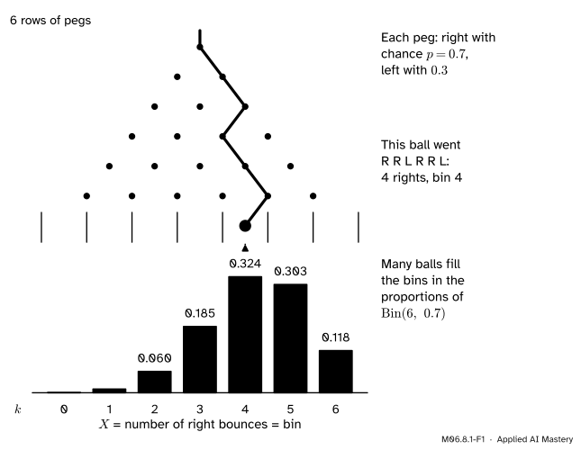
The Galton board of M06.5 tells this story with a ball. Tilt the board so that the ball bounces right with chance \(p\) at every peg. A right bounce is a success, the \(n\) rows of pegs are the \(n\) trials, and the bin where the ball lands is its number of right bounces.
M06.8.1-F1
The binomial story on a tilted Galton board. Each of 6 pegs sends the ball right with chance 0.7. The bin is the number of right bounces, and many balls fill the bins in the proportions of \({\mathrm{Bin}(6, 0.7)}\).
The bars lean to the right because right bounces are more likely, and they peak near \({6 \times 0.7 = 4.2}\). The rest of the lesson finds the height of every bar, the centre and the spread, from the story alone.
Build it up
Step 1. One trial. A random variable that is 1 for a success and 0 for a failure, with \({\Prob(X = 1) = p}\), is a Bernoulli variable, written \({X \sim \mathrm{Bern}(p)}\). It is the indicator of the event “success”. M06.7 found its mean, \({\E[X] = p}\), and its variance, \({p(1 - p)}\).
Step 2. One sequence of trials. Take \({n = 3}\) trials with \({p = 0.9}\), and write S for a success and F for a failure. The trials are independent, so the chance of a whole sequence is the product of the chances of its trials (M06.3.4):
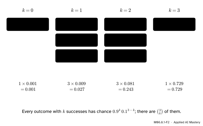
Step 3. Order does not change the chance. The sequences S F S and F S S multiply the same three numbers in another order, so they have the same chance, 0.081. Every sequence with \(k\) successes and \({n - k}\) failures has chance \({p^k (1 - p)^{n-k}}\).
Step 4. Count the sequences. The event “\({X = k}\)” is the set of all sequences with \(k\) successes. To build one, choose which \(k\) of the \(n\) places hold an S. There are \({\binom{n}{k}}\) ways to choose (M06.2.3), so
The 8 outcomes of 3 trials at \({p = 0.9}\), gathered by their number of successes \(k\). Within a column every outcome has the same chance, so the column total is the count times that chance.
The four totals, 0.001, 0.027, 0.243 and 0.729, add up to 1, as the chances of all the outcomes must.
The formal statement
NoteDefinition: Bernoulli and binomial distributions
\(X \sim \mathrm{Bern}(p)\) when \({\Prob(X = 1) = p}\) and \({\Prob(X = 0) = 1 - p}\), for a number \({0 \le p \le 1}\).
\(X \sim \mathrm{Bin}(n, p)\) when \(X\) counts the successes in \(n\) independent trials that each succeed with chance \(p\). Its PMF is
\[
p_X(k) = \binom{n}{k} p^k (1 - p)^{n-k}
\]
for \({k = 0, 1, \ldots, n}\). Its mean is \({\E[X] = np}\) and its variance is \({\mathrm{Var}(X) = np(1 - p)}\).
\(\mathrm{Bern}(p)\) is \({\mathrm{Bin}(1, p)}\), a binomial with one trial. In scipy.stats the two families are bernoulli(p) and binom(n, p), with the same letters.
The PMF sums to 1. By the binomial theorem (M01.8.4), with \({a = p}\) and \({b = 1 - p}\),
That is where the name comes from: the probabilities are the terms of the expansion of a binomial, \({(p + q)^n}\) with \({q = 1 - p}\).
The mean, from indicators. Let \(I_i\) be 1 if trial \(i\) succeeds and 0 if it fails. Each \(I_i\) is \(\mathrm{Bern}(p)\), and the count is their sum:
\[
X = I_1 + I_2 + \cdots + I_n .
\]
Linearity of expectation (M06.7.2) needs no independence and no PMF. Adding \(n\) terms, each \(p\):
The variance, from indicators. The trials are independent, so the variance of the sum is the sum of the variances (M06.7.3), and each is \({p(1 - p)}\):
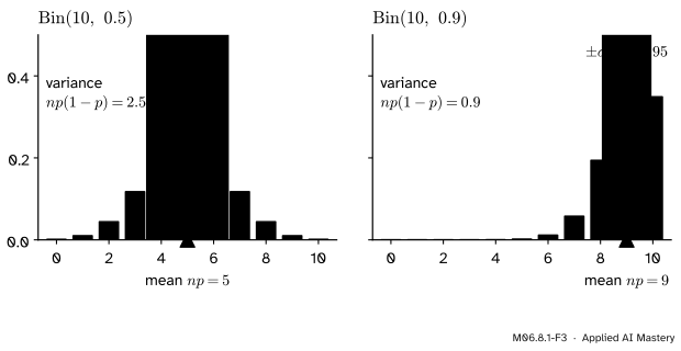
The standard deviation is \({\sigma = \sqrt{np(1 - p)}}\). The spread is largest at \({p = 0.5}\) and shrinks to 0 as \(p\) nears 0 or 1, where almost every trial ends the same way.
M06.8.1-F3
Two binomials with \({n = 10}\). The orange triangle marks the mean \({np}\) and the band reaches one standard deviation either side. With \({p = 0.9}\) the bars crowd against the wall at 10, so the spread is smaller.
Go deeper: the mean straight from the PMF
The indicator argument is short, but the PMF gives the same answer. The identity \({k \binom{n}{k} = n \binom{n-1}{k-1}}\) holds because both sides count the ways to choose a team of \(k\) from \(n\) people and then a captain from the team: the left picks the team first, the right picks the captain first. Then, with \({j = k - 1}\),
The \({k = 0}\) term was dropped because it is 0, and the last sum is the binomial theorem again.
Worked example
A classifier with accuracy 0.9 is tested on 10 independent examples. Find the chance of 10 out of 10, and of 8 or fewer.
Check the story. Each example is a trial; “correct” is a success with \({p = 0.9}\); the examples are independent. So the score is \({X \sim \mathrm{Bin}(10, 0.9)}\).
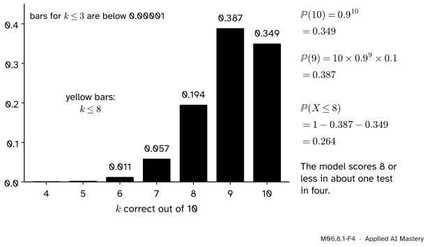
All correct. There is one sequence with 10 successes, so
\[
\Prob(X = 10) = 0.9^{10} = 0.3487 .
\]
Even a model that is right 90% of the time scores 10 out of 10 only about one time in three.
Exactly 9. There are \({\binom{10}{9} = 10}\) places for the single mistake:
The worked example as bars. The yellow bars are the event \({X \le 8}\); their total is 1 minus the two grey bars.
So about one test in four shows 80% accuracy or worse, though the model’s true accuracy is 90%. The mean score is \({np = 9}\) and the standard deviation is \({\sqrt{10 \times 0.9 \times 0.1} = 0.95}\) correct answers: on 10 examples the measured accuracy wobbles by about 10 percentage points.
Code
From scratch, with exact fractions, so that every number can be checked by hand:
import mathfrom fractions import Fractiondef binom_pmf(k, n, p):"""Number of sequences with k successes times the chance of each one."""return math.comb(n, k) * p**k * (1- p) ** (n - k)p = Fraction(9, 10)pmf = [binom_pmf(k, 10, p) for k inrange(11)]all_correct = pmf[10]at_most_8 =1- pmf[9] - pmf[10]mean =sum(k * q for k, q inenumerate(pmf))var =sum(k**2* q for k, q inenumerate(pmf)) - mean**2print("P(X = 10) =", all_correct, "=", round(float(all_correct), 4))print("P(X <= 8) =", at_most_8, "=", round(float(at_most_8), 4))print("total:", sum(pmf), " mean:", mean, " variance:", var)
Next, simulation. Each row of a table of uniform numbers is one test of 10 examples; a number below 0.9 is a correct answer.
import numpy as nprng = np.random.default_rng(seed=0)tests = rng.random((100_000, 10)) <0.9# True means the model got that example rightscores = tests.sum(axis=1)print("share of 10/10:", (scores ==10).mean().round(4), " share of <= 8:", (scores <=8).mean().round(4))print("mean score:", scores.mean().round(3), " variance of the scores:", scores.var().round(3))
share of 10/10: 0.3468   share of <= 8: 0.2642
mean score: 8.997   variance of the scores: 0.901
The simulated shares agree with the exact answers to about two decimal places, as 100,000 tests should. Last, the library: scipy.stats.binom takes n and p in that order.
X.cdf(8) is \({\Prob(X \le 8)}\), the sum of the bars up to 8, which is the calculation above done for us.
Explore
This module’s interactive, the distribution map, lives in lesson M06.8.4. Choose the binomial, set \({n = 10}\) and \({p = 0.9}\), and watch the mean and the one-standard-deviation band; then slide \(p\) towards 0.5 and see the band widen.
Pitfalls
M06.8.1-F5
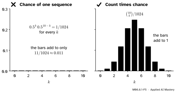
Wrong beside right, for 10 fair flips. On the left each bar is the chance of one particular sequence, and the bars add to almost nothing. Multiplying by the number of sequences, \({\binom{10}{k}}\), gives a distribution.
“The chance of 5 heads in 10 flips is \({0.5^5 \times 0.5^5}\).”
That is the chance of one particular sequence, such as H H H H H T T T T T. The event “5 heads” holds \({\binom{10}{5} = 252}\) sequences, so its chance is \({252/1024 = 0.246}\). A quick check: the bars of a PMF must add to 1.
“Any count of successes is binomial.”
The story needs a fixed number of trials, one chance \(p\) for all of them, and independence. A mini-batch drawn without replacement breaks independence: each draw changes what is left, and the count of positives is hypergeometric (M06.2.4). Near-duplicate examples in a test set break it too, because a model that gets one wrong tends to get its twin wrong.
“The most likely score is exactly the mean.”
The mean \({np}\) need not be a value \(X\) can take, and even when it is, its bar can be small. For \({\mathrm{Bin}(100, 0.5)}\) the mean is 50, yet \({\Prob(X = 50) = 0.0796}\): a score other than 50 is about eleven and a half times as likely as 50 itself.
Check yourself
Recall
1. What is the story of the binomial distribution?
Show answer
\(n\) independent trials, each a success with the same chance \(p\); \(X\) counts the successes.
2. Why does every sequence with \(k\) successes in \(n\) trials have the same chance?
Show answer
By independence its chance is a product of \(k\) factors \(p\) and \({n - k}\) factors \({1 - p}\), and the order of the factors does not change a product.
3. Why do the binomial probabilities add to 1?
Show answer
By the binomial theorem they are the terms of \({(p + (1 - p))^n = 1^n = 1}\).
4. Give the mean and variance of \({\mathrm{Bin}(n, p)}\), and the idea that derives them.
Show answer
Mean \({np}\), variance \({np(1 - p)}\). Write the count as a sum of \(n\) independent \({\mathrm{Bern}(p)}\) indicators, then add their means (linearity) and their variances (independence).
5. For a classifier with accuracy 0.9 on 10 independent examples, what is the chance of a perfect score?
Show answer
\({0.9^{10} = 0.349}\), about one in three.
Exercises
1.★ Four fair coins are flipped. Find the chance of exactly 2 heads, and the mean and variance of the number of heads.
Show solution
\(X \sim \mathrm{Bin}(4, 0.5)\), so \({\Prob(X = 2)} = {\binom{4}{2} \times 0.5^4} = {6/16} = 0.375\), the count of paths to bin 2 of a 4-row Galton board over all 16 paths. The mean is \({np = 2}\) and the variance is \({np(1 - p) = 4 \times 0.25 = 1}\).
2.★★ A spam filter wrongly flags each genuine email with chance 0.2, independently. Five genuine emails arrive. Find the chance that at least one is flagged, and the expected number flagged.
Show solution
The number flagged is \({X \sim \mathrm{Bin}(5, 0.2)}\). By the complement,
and the ratio of the powers is \({p^{k+1} q^{n-k-1} / (p^k q^{n-k}) = p/q}\). Multiplying gives the formula. The bars rise while the ratio is above 1. For \({n = 10}\) and \({p = 0.9}\) the ratio is \({9(10 - k)/(k + 1)}\), which is above 1 when \({90 - 9k > k + 1}\), that is \({k < 8.9}\). So the bars rise up to \({k = 9}\), and the step from 9 to 10 has ratio \({9 \times 1/10 = 0.9 < 1}\). The most likely score is 9, with \({\Prob(X = 9) = 0.387}\).
Summary card
Count the successes in n independent trials of chance p: that count is binomial.
Binomial PMF.\({\binom{n}{k} p^k (1 - p)^{n-k}}\): sequences times chance of each.
Mean and variance.\({np}\) and \({np(1 - p)}\), from a sum of indicators.
SciPy.stats.binom(n, p), stats.bernoulli(p).
Sources and next steps
Sources. Each was opened and checked against this lesson on 14 November 2026.
Hossein Pishro-Nik, Introduction to Probability, Statistics, and Random Processes, Section 3.1.5: the Bernoulli PMF, the binomial PMF for \(n\) coin tosses, and Lemma 3.1, that a binomial is a sum of \(n\) independent Bernoulli variables. Section 3.2.4 derives the Bernoulli variance \({p(1 - p)}\) from \({\E[X^2] - (\E X)^2}\) and the binomial variance \({np(1 - p)}\) by adding the variances of independent Bernoulli variables.
SciPy developers, scipy.stats.binom (SciPy 1.18 reference): the PMF \({\binom{n}{k} p^k (1 - p)^{n-k}}\) for \({k = 0, \ldots, n}\) with shape parameters n and p.
Next.M06.8.2 Geometric and exponential keeps the same trials but asks a different question: not how many successes, but how long until the first.