The expectation of a random variable is the average of its values weighted by their probabilities: the balance point of its distribution and the number a long run of draws settles on. Learn it for PMFs and densities, and for any function of X.
M06.7.1L1 Core25 minIn review (what this means)
The maths and code on this page are checked by automated tests on every change, but an independent reader has not signed it off yet. Spot a mistake or a confusing step? Tell us.
Compute the expectation of a discrete random variable as a probability-weighted sum, and of a continuous one as the integral of x times its density.
Explain the expectation as the balance point of a distribution and as the number that the average of many simulated draws settles on.
Find the expectation of a function g(X) by weighting g(x) with the distribution of X, and prove that rule for a PMF by grouping outcomes.
Show that the expectation of an indicator is the probability of its event, and use it for the accuracy of a classifier.
The question
A die never shows 3.5. Yet roll it ten thousand times, add up the pips and divide by ten thousand, and you get 3.5 to within a few hundredths, every time. Where does that number come from, and why is the same number the training loss that every model in machine learning tries to make small?
Intuition
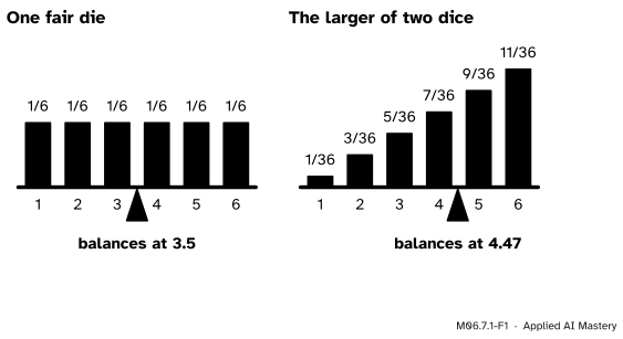
Think of a PMF as a set of weights. Each value \(x\) of the random variable is a position on a beam, and the probability \(p_X(x)\) is the weight hung there. The total weight is 1. The expectation of \(X\), written \(\E[X]\), is the point where that beam balances.
M06.7.1-F1
A PMF as weights on a beam. A fair die balances at 3.5, a value it never shows. The larger of two dice puts more weight on the high values, so its balance point moves right, to \({161/36 \approx 4.47}\).
Two things are worth noticing at once.
The balance point need not be a possible value. The die balances at 3.5, between two faces.
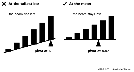
Weight far out pulls hard. On the right, the bar at 6 is tallest, but the beam does not balance there: all the weight to its left pulls the pivot back to 4.47.
The same number has a second meaning, and it is the one that makes it useful: if you draw \(X\) over and over, the average of your draws settles on \(\E[X]\). That is why it is also called the mean of \(X\), and written \(\mu\) for short.
Build it up
Step 1. Average a list of rolls by grouping. Suppose twelve rolls of a die give 3, 6, 1, 4, 4, 2, 6, 5, 3, 6, 2, 4. Their total is 46, so their average is \({46/12 \approx 3.83}\). Add them up a second way, by value: one 1, two 2s, two 3s, three 4s, one 5 and three 6s.
Each value is multiplied by the fraction of rolls that showed it. An average is a weighted sum of the values, with the relative frequencies as weights.
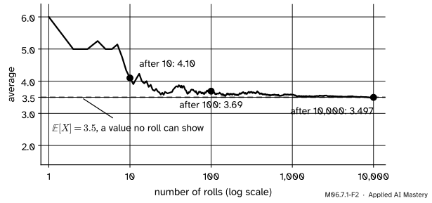
Step 2. Let the rolls run on. As the number of rolls grows, each relative frequency settles down near the probability of its value (the long-run reading of probability, M06.1.3). For a fair die every fraction heads for \(1/6\), so the average heads for
The running average of 10,000 simulated rolls of a fair die (seed 7). Early averages swing widely; later ones hug the dashed line at \(\E[X] = 3.5\).
Step 3. Name it. Replace “fraction of rolls” with “probability” in Step 1 and you have the definition: the expectation is the sum of each value times its probability.
Step 4. Why it is the balance point. Measure each value’s distance from the mean, \({x - \mu}\): negative on the left, positive on the right. A weight \(p_X(x)\) at signed distance \({x - \mu}\) turns the beam with strength \({(x - \mu)\,p_X(x)}\), and the beam balances when these add to 0. At \(\mu = \E[X]\) they do:
The second line splits the sum in two. The third uses the definition of \(\mu\) and the fact that the probabilities add up to 1.
The formal statement
NoteDefinition: expectation
For a discrete random variable \(X\) with PMF \(p_X\), \[
\E[X] = \sum_x x\,p_X(x).
\] For a continuous random variable with density \(f_X\), \[
\E[X] = \int_{-\infty}^{\infty} x\,f_X(x)\,dx .
\]
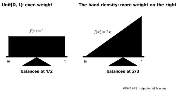
The integral is the sum with its weights spread out. Cut the line into thin strips of width \(\Delta x\); the strip at \(x\) carries probability close to \({f_X(x)\,\Delta x}\) (M06.6.1), so it adds about \({x\,f_X(x)\,\Delta x}\), and as the strips narrow the sum becomes the integral (M04.5).
M06.7.1-F3
A density is weight spread along the line. Even weight on \([0, 1]\) balances in the middle; the hand density \({f(x) = 2x}\) leans right and balances at \(2/3\).
Expectations of functions of \(X\). Often we want the average of something computed from \(X\): its square, a payout, a loss. If \(g\) is a function, \({Y = g(X)}\) is a new random variable, and
\[
\E[g(X)] = \sum_x g(x)\,p_X(x)
\]
for a PMF, or with a density
\[
\E[g(X)] = \int g(x)\,f_X(x)\,dx .
\]
We do not need the PMF of \(Y\) first: weight each \(g(x)\) by the probability of \(x\).
Proof for a PMF, by grouping outcomes. Work on the sample space \(\Omega\), where each outcome \(\omega\) has probability \(\Prob(\{\omega\})\). Averaging any random variable over the outcomes gives its expectation: grouping the outcomes by the value \(y\) they give,
Now group the same outcomes by the value \(x\) of \(X\) instead. On every outcome with \({X(\omega) = x}\) the value of \(Y\) is the same number \(g(x)\), so
Both lines regroup one finite sum (or one absolutely convergent series), so they are equal. The first line also shows \({\E[X]}\)\({= \sum_\omega X(\omega)\,\Prob(\{\omega\})}\), which the next lesson uses.
Go deeper: when an expectation does not exist
The sum or integral must converge absolutely, \({\sum_x \abs{x}\,p_X(x)}\)\({< \infty}\), or we say that \(X\) has no expectation. Take a game that pays \(2^k\) pounds with probability \(2^{-k}\) for \({k = 1, 2, \dots}\). Each term \({2^k \cdot 2^{-k}}\) is 1, so the sum runs off to infinity: the running average of the payouts never settles. Heavy tails like this come back in M06.11.3.
For two dice and \({A = \{\text{the sum is } 7\}}\), \({\E[1_A] = 6/36 = 1/6}\). A classifier’s accuracy is an expectation of this kind: if each test example is correct with probability 0.9, the indicator “correct” has expectation 0.9.
Unif(0, 1). The density is 1 on \([0, 1]\), so \({\E[X]}\)\({= \int_0^1 x\,dx}\)\({= [x^2/2]_0^1}\)\({= 1/2}\).
The hand density. With \({f(x) = 2x}\) on \([0, 1]\),
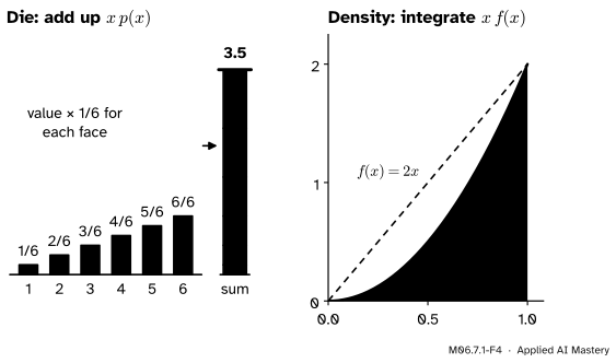
The two computations side by side. For the die, the pieces \({x\,p(x)}\) stack up to 3.5. For the hand density, the area under \({x\,f(x) = 2x^2}\) is \(2/3\).
Code
First from scratch, with a PMF as a dictionary from values to exact fractions.
from fractions import Fractionfrom itertools import productdef expectation(pmf, g=lambda x: x):"""E[g(X)] for a PMF given as {value: probability}."""returnsum(g(x) * p for x, p in pmf.items())die = {k: Fraction(1, 6) for k inrange(1, 7)}# The larger of two dice, built from the 36 equally likely ordered pairs.larger = {}for a, b in product(range(1, 7), repeat=2): larger[max(a, b)] = larger.get(max(a, b), 0) + Fraction(1, 36)# The indicator of "the sum of two dice is 7", as a PMF on {0, 1}.p_seven = Fraction(sum(a + b ==7for a, b in product(range(1, 7), repeat=2)), 36)indicator = {1: p_seven, 0: 1- p_seven}print("E[die] =", expectation(die))print("E[larger of two] =", expectation(larger), "≈", round(float(expectation(larger)), 2))print("E[indicator] =", expectation(indicator))print("E[die squared] =", expectation(die, lambda x: x * x))
Now check by simulation, and do the continuous case with a sum of thin strips. Sampling the hand density uses \(\sqrt{U}\) for a uniform \(U\) (the inverse-CDF method of M06.6.3).
import numpy as nprng = np.random.default_rng(7)rolls = rng.integers(1, 7, size=100_000)print("average of 100,000 rolls:", rolls.mean().round(3))n =100_000# strips for the integral of x * 2x on [0, 1]mid = (np.arange(n) +0.5) / nprint("midpoint sum for the hand density:", (mid *2* mid).sum() / n)draws = np.sqrt(rng.random(100_000))print("average of 100,000 draws of sqrt(U):", draws.mean().round(3))values, probs = np.arange(1, 7), np.full(6, 1/6)print("numpy.average with weights:", np.average(values, weights=probs))
average of 100,000 rolls: 3.507
midpoint sum for the hand density: 0.66666666665
average of 100,000 draws of sqrt(U): 0.667
numpy.average with weights: 3.5000000000000004
numpy.average computes \({\sum a_i w_i / \sum w_i}\), so the weights need not add to 1; with a PMF as the weights it is exactly \(\E[X]\). The simulated averages differ from the exact values in the second or third decimal place, and a different seed moves them by about that much.
Explore
The module’s interactive, the balance beam, is in lesson M06.7.3. You can use it already: raise any bar and watch the pivot, which sits at \(\E[X]\), slide towards it.
Pitfalls
M06.7.1-F5
Wrong beside right. A pivot under the most likely value, 6, lets the beam tip; only the pivot at the mean, 4.47, holds it level.
“The expected value is the value you should expect to see.”
Not in the everyday sense. A die’s expectation, 3.5, never comes up, and the most likely value of the larger of two dice is 6, not its expectation 4.47. The expectation is a long-run average and a balance point. The most likely value has its own name, the mode, and the middle value is the median (M06.5.3); for a lopsided distribution all three differ.
“The mean of a density is where the density is highest.”
The hand density \({2x}\) is highest at \({x = 1}\), but its mean is \(2/3\). Height is probability per unit length, not a vote for one point: the mean comes from \({\int x\,f(x)\,dx}\), which weighs every value \(x\) by its density and also by \(x\) itself.
“A training loss is just a number from the data, nothing to do with expectation.”
The average loss over a data set is an average of draws, and what it estimates is the expected loss over all the data the model might meet. Machine learning minimises the first in the hope of minimising the second; ML01.2 is about the gap between them.
Check yourself
Recall
1. Write the expectation of a discrete \(X\) and of a continuous \(X\).
Show answer
\({\E[X] = \sum_x x\,p_X(x)}\), and \({\E[X] = \int x\,f_X(x)\,dx}\).
2. In the picture of a PMF as weights on a beam, where is \(\E[X]\)?
Show answer
At the balance point: the signed distances \({x - \mu}\), weighted by probability, add to zero there.
3. How do you find \({\E[g(X)]}\) without working out the distribution of \({g(X)}\)?
Show answer
Weight each \({g(x)}\) by the probability (or density) of \(x\): \({\E[g(X)]}\)\({= \sum_x g(x)\,p_X(x)}\).
4. What is the expectation of the indicator of an event \(A\)?
Show answer
\({\Prob(A)}\), because the indicator is 1 with probability \({\Prob(A)}\) and 0 otherwise.
5. What is the mean of the hand density \({f(x) = 2x}\) on \([0, 1]\)?
Show answer
\({\int_0^1 x \cdot 2x\,dx}\)\({= 2/3}\).
Exercises
1.★ You roll a die and win £10 on a six and lose £1 otherwise. What are your expected winnings per game?
Show solution
The winnings \(W\) are 10 with probability \(1/6\) and \(-1\) with probability \(5/6\), so \({\E[W]}\)\({= 10 \cdot \tfrac16 - 1 \cdot \tfrac56}\)\({= \tfrac56}\)\({\approx 0.83}\) pounds per game.
2.★★ For the hand density \({f(x) = 2x}\) on \((0, 1]\), find \({\E[X^2]}\) and \({\E[1/X]}\). Is \({\E[1/X]}\) equal to \({1/\E[X]}\)?
Show solution
\({\E[X^2]}\)\({= \int_0^1 x^2 \cdot 2x\,dx}\)\({= [x^4/2]_0^1}\)\({= 1/2}\). \({\E[1/X]}\)\({= \int_0^1 \tfrac1x \cdot 2x\,dx}\)\({= \int_0^1 2\,dx}\)\({= 2}\). But \({1/\E[X] = 1/(2/3) = 1.5}\), so no: the expectation of a function is not the function of the expectation. The next lesson returns to this.
3.★★★ The waiting time \(T\) has density \({\lambda e^{-\lambda t}}\) for \({t \ge 0}\), with rate \({\lambda = 0.5}\) per minute. Show that \({\E[T] = 1/\lambda = 2}\) minutes.
Show solution
\({\E[T]}\)\({= \int_0^\infty t\,\lambda e^{-\lambda t}\,dt}\). Integrate by parts (M04.7) with \({u = t}\) and \({dv}\)\({= \lambda e^{-\lambda t}\,dt}\), so \({du = dt}\) and \({v = -e^{-\lambda t}}\). Up to a limit \(b\),
As \({b \to \infty}\), \({b e^{-\lambda b} \to 0}\) and \({e^{-\lambda b} \to 0}\), leaving \({1/\lambda}\). With \({\lambda = 0.5}\) that is 2 minutes.
Summary card
The expectation is where the distribution balances, and what long-run averages settle on.
A function of \(X\):\({\E[g(X)]}\)\({= \sum_x g(x)\,p_X(x)}\), with no new PMF needed.
Indicator:\({\E[1_A] = \Prob(A)}\).
Running examples: a die 3.5, Unif(0, 1) 1/2, the hand density 2/3.
Sources and next steps
Sources. Each was opened and checked against this lesson on 14 November 2026.
Jeremy Orloff and Jonathan Bloom, Reading 4b: Discrete Random Variables: Expected Value, MIT OpenCourseWare 18.05, Spring 2022. Section 2 defines \({\E[X] = \sum p(x_j)\,x_j}\) and notes that it need not be a possible value; Section 2.1 reads it as the centre of mass, “the point at which the distribution would balance”; Section 2.3 gives \({\E[h(X)]}\)\({= \sum h(x_j)\,p(x_j)}\) and works \({\E[X^2] = 15.167}\) for a die.
Charles M. Grinstead and J. Laurie Snell, Introduction to Probability, second edition. Section 6.1, Definition 6.1 (expected value, with absolute convergence) and Theorem 6.1 (the expectation of \({\phi(X)}\), proved by grouping values); Section 6.3, Definition 6.4 (the continuous case).
Hossein Pishro-Nik, Expected Value and Variance, Introduction to Probability, Statistics, and Random Processes, Section 4.1.2: the continuous expectation and its version for \({g(X)}\) (Equation 4.3), with the uniform mean \({(a + b)/2}\) and the density \({2x}\) worked to a mean of \(2/3\).
NumPy, numpy.average: the weighted average \({\sum a\,w / \sum w}\), with weights that need not sum to 1.