Average n independent draws and you get a new random variable, the sample mean. Derive that its expectation is the mean μ and its variance is σ²/n, so its spread shrinks like 1/√n, and see it on dice and on a test-set accuracy.
M06.11.1L1 Core25 minIn review (what this means)
The maths and code on this page are checked by automated tests on every change, but an independent reader has not signed it off yet. Spot a mistake or a confusing step? Tell us.
Explain why the average of n random draws is itself a random variable with its own distribution.
Derive E[X̄ₙ] = μ and Var(X̄ₙ) = σ²/n for independent, identically distributed draws, naming the rule used at each step.
Use the standard deviation σ/√n to say how much an average wanders, and how much more data narrows it.
Build the exact distribution of the mean of n dice by repeated convolution with numpy.convolve, and check it by simulation.
The question
A classifier is right on 90% of all the emails it will ever see. You measure it on a test set of 100 emails and get 0.87; a colleague measures it on another 100 and gets 0.93. Neither of you is wrong: the score is an average of 100 random results, so it is random too. How far should such an average wander from the truth, and how much does a bigger test set help?
Intuition
Draw \(n\) values at random and average them. That gives one number. Draw a fresh sample and average again: you get a different number. So the average is not fixed. It is a random variable, a number that depends on the outcome of a chance experiment (M06.5.1), and like every random variable it has a distribution.
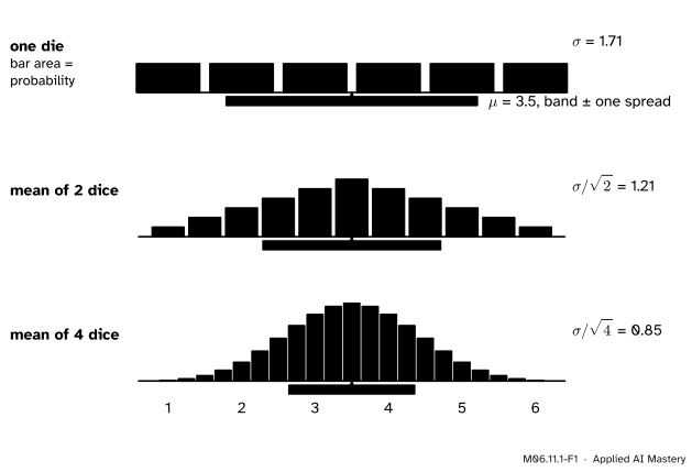
The picture shows that distribution, worked out exactly, for the average of 1, 2 and 4 fair dice.
M06.11.1-F1
The exact distribution of the average of 1, 2 and 4 dice. The bars are drawn so that each bar’s area is its probability. The centre stays at 3.5; the spread shrinks from 1.71 to 1.21 to 0.85.
Two things stand out. The centre does not move: averages of dice balance at 3.5, like a single die. And the spread shrinks: extreme averages need every die to be extreme at once, which is rare, so the values crowd towards the middle. This lesson puts numbers on both facts.
Build it up
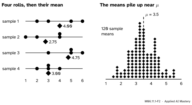
Step 1. One sample, one mean. Roll four dice, say 2, 5, 3 and 6. Their sample mean is \({(2 + 5 + 3 + 6)/4 = 4}\). That is one value of the random variable.
Step 2. Many samples, many means. Repeat with fresh dice and the mean changes: 2.75, 4.75, 3. Pile up the means of many samples and a shape appears.
M06.11.1-F2
Left: each sample of four rolls (blue) gives one mean (vermillion). Right: the means of 120 simulated samples, stacked, pile up near \({\mu = 3.5}\).
Step 3. The exact distribution. A pile of simulated means is only an estimate. The exact distribution comes from the sum \({S_n = X_1 + \dots + X_n}\). For independent dice its PMF is a convolution, adding products along diagonals (M06.5.4). For two dice it is the triangle \({1, 2, \dots, 6, \dots, 2, 1}\) over 36, and the mean \({S_2/2}\) takes the same probabilities at half the values. Convolve twice more for four dice: \({S_4 = 14}\) in 146 of the 1,296 ordered rolls, so
Step 4. Name what we see. The centre is the same for every \(n\). The spread is not. To say by how much it shrinks we need the expectation and the variance of the mean.
The formal statement
NoteDefinition and result: the sample mean
Let \(X_1, \dots, X_n\) be independent and identically distributed (i.i.d.): independent, and each with the same distribution, of mean \(\mu\) and variance \(\sigma^2\). Their sample mean is
The variance. Two rules from M06.7.3: a constant factor comes out squared, \({\operatorname{Var}(aY)}\)\({= a^2 \operatorname{Var}(Y)}\), and the variances of independent variables add. Then
The first line uses \({a = 1/n}\), the second uses independence, and the third uses that every \(X_i\) has the same variance. Take the square root for the standard deviation, \({\sigma/\sqrt{n}}\).
So the sum and the mean pull in opposite directions. The sum’s spread grows like \({\sigma\sqrt{n}}\), the square-root law of M06.7.3; dividing by \(n\) turns that into \({\sigma/\sqrt{n}}\).
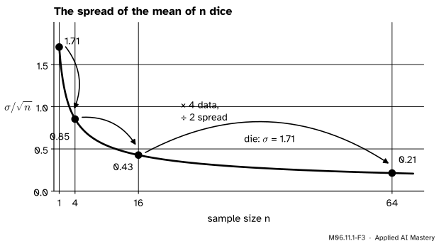
M06.11.1-F3
The standard deviation of the mean of \(n\) dice. Each time the data are multiplied by 4 the spread halves: 1.71, 0.85, 0.43, 0.21.
Because of the square root, four times the data halves the spread. Halving it again needs sixteen times the data. Every extra digit of precision costs a hundred times more draws.
Go deeper: what independence buys
Only the variance step used independence. Without it, \({\operatorname{Var}(S_n)}\) picks up a covariance for every pair (M06.10.2). In the extreme case every \(X_i\) is the same draw, so \({\bar{X}_n = X_1}\) and its variance is \(\sigma^2\), not \({\sigma^2/n}\): averaging copies of one value teaches nothing new. The expectation step never needed independence, so \(\E[\bar{X}_n] = \mu\) holds either way.
Worked example
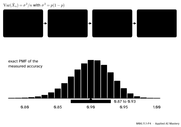
Accuracy on a test set. A classifier answers each example correctly with probability 0.9, independently. Let \({X_i = 1}\) if example \(i\) is right and 0 if not. Each \(X_i\) is a Bernoulli variable, so \({\mu = 0.9}\) and \({\sigma^2}\)\({= p(1 - p)}\)\({= 0.9 \times 0.1}\)\({= 0.09}\) (M06.7.3). The measured accuracy on 100 examples, the test score of ML01.2.3, is the sample mean \({\bar{X}_{100}}\).
M06.11.1-F4
From one example to the score on 100 examples: the variance divides by 100, so the spread is \({\sqrt{0.0009} = 0.03}\). Below, the exact PMF of the measured accuracy, with the band 0.87 to 0.93.
So scores of 0.87 and 0.93 are each one standard deviation from the truth: ordinary luck of the draw. With 400 examples the spread halves to \({0.3/20 = 0.015}\). To reach 0.01 we need \({0.3/\sqrt{n} = 0.01}\), so \({\sqrt{n} = 30}\) and \({n = 900}\).
Frontier note: error bars on reported results
Machine-learning papers often train a model several times with different random seeds and report the mean score with an error bar. If the runs are independent and one run’s score has standard deviation \(s\), the mean of \(k\) runs has standard deviation \({s/\sqrt{k}}\), called the standard error. Five seeds shrink the error bar of the mean to about 45% of a single run’s spread (\({1/\sqrt{5} \approx 0.447}\)). Statistics courses (S02.1, S02.2) estimate \(s\) from the runs themselves and turn the error bar into a confidence interval (S02.4).
Four dice. For one die \({\sigma = \sqrt{35/12} \approx 1.71}\), so the mean of four dice has standard deviation \({1.71/2 \approx 0.85}\), the band in the anchor figure.
Code
From scratch: the exact distribution of the mean of \(n\) dice by repeated convolution, then its mean and standard deviation.
import numpy as npface = np.full(6, 1/6) # P(die = 1), ..., P(die = 6)def mean_of_dice(n):"""Values and exact probabilities of the average of n fair dice.""" pmf = np.array([1.0])for _ inrange(n): pmf = np.convolve(pmf, face) # one more die: add products along diagonals values = np.arange(n, 6* n +1) / nreturn values, pmffor n in (1, 2, 4, 16): v, p = mean_of_dice(n) mu = np.sum(v * p) sd = np.sqrt(np.sum((v - mu) **2* p))print(f"n = {n:2}: mean {mu:.3f}, sd {sd:.4f}, sigma/sqrt(n) = {np.sqrt(35/12/ n):.4f}")v4, p4 = mean_of_dice(4)print("P(mean of 4 dice = 3.5) =", round(p4[v4 ==3.5][0] *1296), "/ 1296")
n =  1: mean 3.500, sd 1.7078, sigma/sqrt(n) = 1.7078
n =  2: mean 3.500, sd 1.2076, sigma/sqrt(n) = 1.2076
n =  4: mean 3.500, sd 0.8539, sigma/sqrt(n) = 0.8539
n = 16: mean 3.500, sd 0.4270, sigma/sqrt(n) = 0.4270
P(mean of 4 dice = 3.5) = 146 / 1296
Now the test set, simulated: 20,000 test sets of 100 examples, each right with probability 0.9.
rng = np.random.default_rng(7)correct = rng.random((20_000, 100)) <0.9# one row per test setscores = correct.mean(axis=1) # 20,000 measured accuraciesprint("mean of the scores:", scores.mean().round(4))print("sd of the scores: ", scores.std().round(4), " theory sqrt(0.09/100) =", np.sqrt(0.09/100))from scipy import statsprint("scipy: sd of Bin(100, 0.9) / 100 =", stats.binom(100, 0.9).std() /100)
mean of the scores: 0.9003
sd of the scores:   0.0302   theory sqrt(0.09/100) = 0.03
scipy: sd of Bin(100, 0.9) / 100 = 0.03
The simulated scores agree with \({\sigma/\sqrt{n} = 0.03}\) to within simulation noise (the last digit may differ on another machine). The number correct out of 100 is \({\mathrm{Bin}(100, 0.9)}\) (M06.8.1), so scipy gives the same spread once divided by 100.
Explore
The module’s interactive, the sample-mean machine, lives in lesson M06.11.3. Try this there: pick the die, set \({n = 1}\) and draw a few hundred means, then do the same at \({n = 4}\) and \({n = 16}\). The read-out gives the spread of your means beside \({\sigma/\sqrt{n}}\): about 1.71, 0.85 and 0.43.
Pitfalls
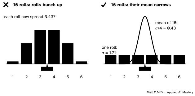
M06.11.1-F5
Wrong beside right. Rolling more dice does not change how one roll is spread (left, wrong). What narrows is the distribution of their mean (right).
“With more data, the data become less spread out.”
Each roll still has standard deviation 1.71, however many you make; a histogram of 16,000 rolls is as flat as one of 16. What shrinks is the spread of the average. In machine learning the same holds: a bigger test set does not make examples easier, it makes the score steadier.
“The spread of the mean falls like 1/n.”
It falls like \({1/\sqrt{n}}\), because the variance falls like \(1/n\) and the standard deviation is its square root. With 100 test examples the spread is \({0.3/\sqrt{100} = 0.03}\), not \({0.3/100 = 0.003}\). Promising ten times the precision for ten times the data overstates it by a factor of about three.
“Any n values will do.”
The \({\sigma^2/n}\) needs independence. A test set with 100 near-copies of the same email behaves like one example, not 100: the copies are right or wrong together, and the score is as noisy as a single answer. Duplicates between training and test data, or many photos of one person, quietly break the \({1/\sqrt{n}}\) promise.
Check yourself
Recall
1. Why is a sample mean a random variable?
Show answer
It is computed from random draws, so a fresh sample gives a different value; it is a number that depends on the outcome of the experiment.
2. For i.i.d. draws with mean \(\mu\) and variance \(\sigma^2\), what are \({\E[\bar{X}_n]}\) and \({\operatorname{Var}(\bar{X}_n)}\)?
Show answer
\({\E[\bar{X}_n] = \mu}\) and \({\operatorname{Var}(\bar{X}_n)}\)\({= \sigma^2/n}\), so the standard deviation is \({\sigma/\sqrt{n}}\).
3. Which step of the derivation needs independence?
Show answer
The variance step, where the variances of the \(X_i\) add. The expectation step uses linearity only.
4. How much data does it take to halve the spread of an average?
Show answer
Four times as much, because \({\sigma/\sqrt{4n}}\)\({= \tfrac12\,\sigma/\sqrt{n}}\).
5. What is the standard deviation of the accuracy measured on 100 examples when the true accuracy is 0.9?
Show answer
\({\sqrt{0.9 \times 0.1/100} = 0.03}\).
Exercises
1.★ Find the standard deviation of the mean of 9 dice, and the number of dice whose mean has standard deviation about 0.17.
Show solution
\({\sigma/\sqrt{9}}\)\({= 1.708/3}\)\({\approx 0.569}\). For about 0.17 we need \({\sqrt{n}}\)\({\approx 1.708/0.17}\)\({\approx 10}\), so \({n = 100}\) dice (exactly \({1.708/10 \approx 0.171}\)).
2.★★ How many test examples are needed for the measured accuracy to have standard deviation 0.01 when the true accuracy is 0.9? And when it is 0.5?
Show solution
We need \({p(1 - p)/n = 0.01^2 = 0.0001}\). At \({p = 0.9}\), \({n = 0.09/0.0001 = 900}\). At \({p = 0.5}\), \({n = 0.25/0.0001 = 2{,}500}\). The Bernoulli variance \({p(1 - p)}\) is largest at \({p = 0.5}\), so a score near one half needs the most data for the same precision.
3.★★★ List the PMF of the mean of two dice and compute its variance directly from the list. Check that you get \({\sigma^2/2 = 35/24}\).
Show solution
\({\bar{X}_2 = S_2/2}\) takes the values \({1, 1.5, \dots, 6}\) with probabilities \({1, 2, 3, 4, 5, 6, 5, 4, 3, 2, 1}\) over 36. Its mean is 3.5, and \({(\bar{x} - 3.5)^2 = (s - 7)^2/4}\). So
Four times the data halves the spread. Accuracy 0.9 on 100 examples: \({\pm 0.03}\).
Sources and next steps
Sources. Each was opened and checked against this lesson on 14 November 2026.
Hossein Pishro-Nik, Law of Large Numbers, Section 7.1.1 of Introduction to Probability, Statistics, and Random Processes: the definition of the sample mean of i.i.d. variables, with \({\E[\bar{X}] = \E[X]}\) and \({\operatorname{Var}(\bar{X})}\)\({= \operatorname{Var}(X)/n}\) derived from linearity and independence.
Jeremy Orloff and Jonathan Bloom, Reading 6b: Central Limit Theorem and the Law of Large Numbers, MIT OpenCourseWare 18.05, Spring 2022. Section 3 notes that the average is itself a random variable; Section 5.2 lists \({\E[\bar{X}_n] = \mu}\), \({\operatorname{Var}(\bar{X}_n)}\)\({= \sigma^2/n}\) and \({\sigma_{\bar{X}_n} = \sigma/\sqrt{n}}\).
Charles M. Grinstead and J. Laurie Snell, Introduction to Probability, second edition, Section 8.1: the proof of Theorem 8.2 computes \({V(S_n) = n\sigma^2}\) and \({V(S_n/n) = \sigma^2/n}\).
NumPy, numpy.convolve: the discrete convolution, which its notes connect to the distribution of a sum of independent random variables.