Split the sample space into pieces, find the chance of an event inside each piece, weight each by the size of its piece and add. Derive the law of total probability, see it as adding strips of area or leaves of a tree, and use it on an inbox and a medical test.
M06.3.3L1 Core25 minIn review (what this means)
The maths and code on this page are checked by automated tests on every change, but an independent reader has not signed it off yet. Spot a mistake or a confusing step? Tell us.
Define a partition of the sample space and recognise one in a word problem.
Derive the law of total probability from additivity and the multiplication rule.
Explain why P(A) is a weighted average of the conditional probabilities P(A | B_i), and so lies between the smallest and the largest of them.
Compute a total probability from a tree, from an area diagram and from a table of natural frequencies.
Check a total probability by a two-stage simulation in NumPy.
The question
A condition affects 1% of people. A test for it comes back positive for 90% of the people who have it, and also, wrongly, for 10% of the people who do not. If everybody is tested, what share of all the results will be positive? It is not 90%, and it is not 10%. A hospital planning follow-up appointments, and a team estimating how many alerts a fraud model will raise, both need this number.
From the last lesson
1. State the multiplication rule.
Show answer
\({\Prob(A \cap B) = \Prob(B)\,\Prob(A \mid B)}\), and equally \({\Prob(A)\,\Prob(B \mid A)}\).
2. What is the chance that a mini-batch of 4 from 10 examples, 3 positive, has no positive, written as a product?
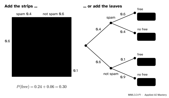
Some probabilities are hard to see directly but easy to find piece by piece. In the inbox of M06.3.1, what share of emails contain “free”? Suppose you know it only by group: 60% of the spam contain it, and 10% of the rest. Spam is 40% of the inbox.
M06.3.3-F1
Two pictures of one sum. The yellow pieces of the square are the leaves of the tree that end in “free”. Add them and you have the chance of “free”.
Every email is either spam or not, never both. So the emails with “free” fall into two separate heaps: spam with “free” and other email with “free”. The multiplication rule gives each heap, \({0.4 \times 0.6 = 0.24}\) and \({0.6 \times 0.1 = 0.06}\), and the whole is their sum, 0.30. That is what the count of 30 emails in 100 said.
Build it up
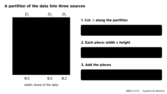
Nothing limits this to two groups. Suppose a model’s training data come from three sources. Half come from the first source, 30% from the second and 20% from the third, and the model’s error rate on them is 0.1, 0.2 and 0.4. Pick an example at random: what is the chance that the model gets it wrong?
Step 1. Cut along the groups. Every example comes from exactly one source. So the set \(A\) of errors splits into three pieces with no overlap: errors on source 1, on source 2, on source 3.
Step 2. Find each piece. A piece is “from source \(i\) and wrong”. By the multiplication rule its chance is the share of the source times the error rate on it: a strip’s width times its height.
Step 3. Add the pieces. They do not overlap, so their chances add.
M06.3.3-F2
The law of total probability in three steps. The groups must cover everything and must not overlap; then the pieces of \(A\) add up to \(A\).
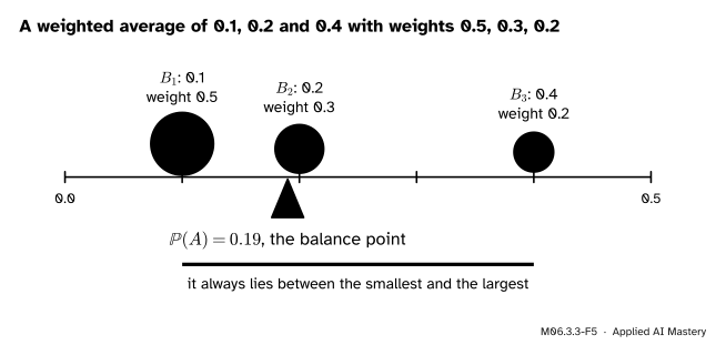
The error rate over all the data is 0.19. It sits between the best source (0.1) and the worst (0.4), nearer the best, because the best source supplies half the data.
The formal statement
NoteDefinition: partition
Events \({B_1, \dots, B_k}\) form a partition of \(\Omega\) if they are pairwise disjoint (no two share an outcome) and cover\(\Omega\) (their union is \(\Omega\)). Then every outcome lies in exactly one \(B_i\).
The simplest partition is an event and its complement, \(B\) and \(B^c\).
NoteThe law of total probability
If \({B_1, \dots, B_k}\) is a partition of \(\Omega\) and every \({\Prob(B_i) > 0}\), then for any event \(A\)
Multiply. By the multiplication rule, each \({\Prob(A \cap B_i)} = {\Prob(A \mid B_i)\,\Prob(B_i)}\). Put that into the sum and the law appears.
In a tree, the \(B_i\) are the branches of the first stage and \(A\) is an outcome of the second. The law says: find every leaf that ends in \(A\), multiply along each path, and add.
A weighted average. The weights \({\Prob(B_1), \dots, \Prob(B_k)}\) are never negative and add to \({\Prob(\Omega) = 1}\), by additivity again. So \(\Prob(A)\) is a weighted average of the conditional probabilities \({\Prob(A \mid B_i)}\). A weighted average lies between the smallest and the largest of the things it averages. To see it, let \(m\) be the smallest \({\Prob(A \mid B_i)}\). Each term is at least \(m\) times its weight, so
The same steps with the largest value \(M\) and “at most” give \({\Prob(A) \le M}\).
M06.3.3-F5
\(\Prob(A)\) is where the line balances when each conditional chance carries its weight. Heavy weights pull it towards themselves.
One consequence is worth knowing by heart. With the partition \(B\), \(B^c\), the chance of \(A\) lies between \({\Prob(A \mid B)}\) and \({\Prob(A \mid B^c)}\). Learning \(B\) moves your belief one way and learning \(B^c\) moves it the other way, never both in the same direction.
Go deeper: what if some piece has probability 0?
If \({\Prob(B_i) = 0}\) then \({\Prob(A \mid B_i)}\) is not defined, but the term it would sit in is not needed: \({\Prob(A \cap B_i) \le \Prob(B_i) = 0}\), so that piece of \(A\) adds nothing. Drop such pieces from the sum, or read their terms as 0. The law also holds for a countable partition \({B_1, B_2, \dots}\), with the same proof, because the additivity axiom holds for countably many disjoint events (M06.1.3).
Worked example
The test. A condition affects 1% of people. The test is positive for 90% of those with it and for 10% of those without. Find the chance that a person picked at random tests positive.
Pick the partition. Each person has the condition (\(C\)) or not (\(C^c\)), so \(C\), \(C^c\) is a partition, with \({\Prob(C) = 0.01}\) and \({\Prob(C^c) = 0.99}\).
Read off the conditional chances.\({\Prob(\text{pos} \mid C) = 0.9}\) and \({\Prob(\text{pos} \mid C^c) = 0.1}\).
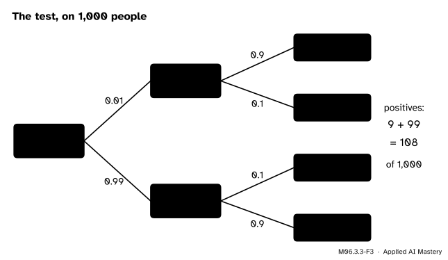
Check with people. Imagine 1,000 people. The tree in the figure splits them: 10 have the condition and 9 of those test positive; 990 do not and 99 of those test positive.
M06.3.3-F3
The same calculation with counts. The yellow leaves are all the positives: 9 true and 99 false, 108 in all.
So 108 of every 1,000 results are positive, a share of 0.108. It lies between 0.1 and 0.9, as it must, and very near 0.1, because 99% of the weight sits on the people without the condition. Most of the positives, 99 of 108, come from people who do not have it. Lesson M06.4.2 turns that remark into Bayes’ rule.
Code
From scratch: a function of the weights and the conditional chances, run on the inbox, the test and the three data sources.
from fractions import Fraction as Fdef total_probability(weights, conditionals):"""P(A) = sum of P(A | B_i) P(B_i) over a partition B_1, ..., B_k."""assertsum(weights) ==1, "the B_i must cover everything, once"returnsum(c * w for c, w inzip(conditionals, weights))p_free = total_probability([F(4, 10), F(6, 10)], [F(6, 10), F(1, 10)])p_pos = total_probability([F(1, 100), F(99, 100)], [F(9, 10), F(1, 10)])p_err = total_probability([F(5, 10), F(3, 10), F(2, 10)], [F(1, 10), F(2, 10), F(4, 10)])print("P(free) =", p_free, " P(positive) =", p_pos, " P(error) =", p_err)
Exact fractions keep \(0.108\) exact: \(108/1000\), which Python shows as \(27/250\).
Now simulate the test in two stages, the way the tree reads. First decide who has the condition, then draw each test result with the chance that belongs to that person.
import numpy as nprng = np.random.default_rng(seed=11)n =1_000_000has_condition = rng.random(n) <0.01# stage 1chance_positive = np.where(has_condition, 0.9, 0.1) # the branch each person is onpositive = rng.random(n) < chance_positive # stage 2print("simulated P(positive):", positive.mean())print("people with the condition:", has_condition.sum()," of whom positive:", positive[has_condition].sum())
simulated P(positive): 0.107885
people with the condition: 10064  of whom positive: 9040
The simulated share is within a whisker of \(0.108\); the last digits depend on the seed.
Explore
M06.3-X1
Zoom-in square
Set the width of the \(B\) strip and the share of \(A\) in each strip with the sliders, or drag the cuts. The four areas, the tree and \(\Prob(A)\) change together, and the dashed line marks \(\Prob(A)\). Try the presets, then make the two shares equal and read what the read-out says about independence.
Pitfalls
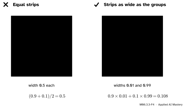
M06.3.3-F4
Wrong beside right. Averaging 0.9 and 0.1 plainly treats the two groups as equally large. The groups are 1% and 99% of people, so the yellow area is 0.108, not 0.5.
“P(positive) is the average of P(positive | condition) and P(positive | no condition).”
Only a weighted average, with the sizes of the groups as weights. The plain average gives 0.5 here, nearly five times the truth. The same slip happens with classifiers: overall accuracy is the average of the per-class accuracies weighted by how common each class is, which is why a model can score 99% on rare-disease data by ignoring the disease.
“Add P(A | B) and P(A | not B) to get P(A).”
Without the weights the sum can exceed 1: for the test, \({0.9 + 0.1 = 1}\) already, and other numbers go past it. Each conditional chance must be multiplied by the probability of its condition.
“Any list of groups will do as the B_i.”
The groups must not overlap and must cover everything. “Spam” and “contains a link” overlap, so adding the chances of “free” through both would count some emails twice. If the weights do not add to 1, the list is not a partition.
Check yourself
Recall
1. What two conditions make \({B_1, \dots, B_k}\) a partition of \(\Omega\)?
Show answer
They are pairwise disjoint, and their union is \(\Omega\): every outcome lies in exactly one of them.
2. State the law of total probability.
Show answer
\({\Prob(A) = \sum_i \Prob(A \mid B_i)\,\Prob(B_i)}\) for a partition \({B_1, \dots, B_k}\) with every \({\Prob(B_i) > 0}\).
3. Which two earlier results does its derivation use?
Show answer
Additivity over the disjoint pieces \({A \cap B_i}\), and the multiplication rule for each piece.
4. In the inbox, how is \({\Prob(\text{free}) = 0.30}\) built?
Show answer
\({0.6} \times {0.4} + {0.1} \times {0.6} = {0.24} + {0.06} = {0.30}\): the share of spam with “free” times the share of spam, plus the same for the other emails.
5. Why must \({\Prob(A)}\) lie between \({\Prob(A \mid B)}\) and \({\Prob(A \mid B^c)}\)?
Show answer
Because it is their weighted average, with weights \({\Prob(B)}\) and \({\Prob(B^c)}\) that are not negative and add to 1.
Exercises
1.★ Two dice are rolled. Use the first die as a partition to find the chance that the sum is 7.
Show solution
Let \(B_i\) be “the first die shows \(i\)”, for \({i = 1, \dots, 6}\), each with chance \(1/6\). Whatever the first die shows, exactly one face of the second makes the sum 7, so \({\Prob(\text{sum } 7 \mid B_i) = 1/6}\) for every \(i\). The law gives \({6 \times (1/6)(1/6) = 1/6}\), which matches the 6 cells of the diagonal out of 36.
2.★★ A classifier is right on 95% of the cats and 80% of the dogs in a test set that is 70% cats and 30% dogs. Find its overall accuracy. What would it be on a set that is half cats and half dogs?
Show solution
With the partition cat, dog: \({0.95} \times {0.7} + {0.80} \times {0.3} = {0.665} + {0.24} = {0.905}\). On a balanced set: \({0.95} \times {0.5} + {0.80} \times {0.5} = {0.875}\). The model has not changed; only the weights have. A single accuracy figure depends on the mix of classes it was measured on.
3.★★★ Let \({0 < \Prob(B) < 1}\). Show that if \({\Prob(A \mid B) = \Prob(A \mid B^c)}\), then \({\Prob(A)}\) equals that common value. Then show the converse: if \({\Prob(A) = \Prob(A \mid B)}\) then \({\Prob(A \mid B^c) = \Prob(A \mid B)}\).
Show solution
Write \(q\) for the common value and \(b\) for \(\Prob(B)\). The law gives \({\Prob(A) = q\,b + q\,(1 - b) = q}\). For the converse, write \({p = \Prob(A \mid B)}\) and \({r = \Prob(A \mid B^c)}\). The law says \({\Prob(A) = p\,b + r\,(1 - b)}\). If this equals \(p\), then \({r\,(1 - b) = p - p\,b = p\,(1 - b)}\), and dividing by \({1 - b > 0}\) gives \({r = p}\). So learning \(B\) leaves the chance of \(A\) unchanged exactly when the two shares are level: this is independence, the next lesson.
Summary card
Cut \(A\) along a partition, find each piece with the multiplication rule, and add.
M06.3.3-F1
Add the strips, or add the leaves.
Law.\({\Prob(A) = \sum_i \Prob(A \mid B_i)\,\Prob(B_i)}\) over a partition.
Weighted average. So \(\Prob(A)\) lies between the smallest and largest \({\Prob(A \mid B_i)}\).
Sources. Each was opened and checked against this lesson on 14 November 2026.
Hossein Pishro-Nik, Introduction to Probability, Statistics, and Random Processes, Section 1.4.2, Law of Total Probability: for a partition \({B_1, B_2, \dots}\) of the sample space, \({\Prob(A)} = {\sum_i \Prob(A \cap B_i)} = {\sum_i \Prob(A \mid B_i)\,\Prob(B_i)}\).
Jeremy Orloff and Jonathan Bloom, Reading 3: Conditional Probability, Independence and Bayes’ Theorem, MIT OpenCourseWare 18.05, Spring 2022. Section 4 states the law for a sample space divided into disjoint pieces, as equation (3); section 5 reads it off a tree as the sum over the paths that end in the event.
Chris Piech, Law of Total Probability, Probability for Computer Scientists (Stanford CS109 reader): the law for mutually exclusive events that between them contain every outcome.
Next.M06.3.4 Independence studies the case where the shares are level, and M06.4 turns the tree round with Bayes’ rule, using totals of this kind as denominators: \({\Prob(\text{free}) = 0.30}\) in M06.4.1 and \({\Prob(\text{pos}) = 0.108}\) in M06.4.2.