The expectation of a sum is the sum of the expectations, with no independence needed. Prove it over the sample space, count with indicators to get the expected heads in n flips and the expected shared birthdays among 23 people, and see where products and nonlinear functions break the pattern.
M06.7.2L1 Core25 minIn review (what this means)
The maths and code on this page are checked by automated tests on every change, but an independent reader has not signed it off yet. Spot a mistake or a confusing step? Tell us.
Prove that E[aX + b] = aE[X] + b and E[X + Y] = E[X] + E[Y] by summing over the sample space, and explain why independence is not needed.
Find the expected value of a count by writing it as a sum of indicators, for heads in n flips and for pairs of people who share a birthday.
Prove that E[XY] = E[X]E[Y] for independent X and Y, and give a dependent pair for which it fails.
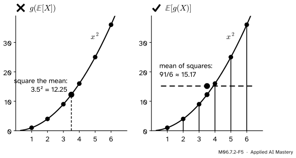
Explain with a picture why E[g(X)] differs from g(E[X]) when g is not a straight line, and check each result by simulation.
The question
Twenty-three people are in a room. On average, how many pairs of them share a birthday? Working out the full distribution of that count is a tangle of overlapping cases. Yet the answer, \({253/365 \approx 0.69}\), takes two lines, by a rule that also tells you the expected number of heads in a thousand flips, the expected accuracy of a classifier on a test set, and the expected loss over a mini-batch.
From the last lesson
1. What is the expectation of one fair die, and is it a value the die can show?
Show answer
\({21/6 = 3.5}\). No: it is the balance point of the six equal weights, between two faces.
2. How do you compute \({\E[g(X)]}\) for a discrete \(X\)?
Show answer
\({\E[g(X)]}\)\({= \sum_x g(x)\,p_X(x)}\): weight each \(g(x)\) by the probability of \(x\).
Intuition
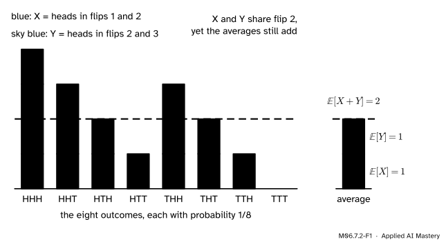
Flip three fair coins. Let \(X\) count the heads among flips 1 and 2, and \(Y\) the heads among flips 2 and 3. The two counts share flip 2, so they are not independent: if \(X = 2\), flip 2 was a head, which makes a large \(Y\) more likely.
Draw each of the eight equally likely outcomes as a column: \(X\) blue blocks at the bottom, \(Y\) sky-blue blocks on top. The height of a column is \({X + Y}\) for that outcome.
M06.7.2-F1
The average height of the stacks is the average of the blue parts plus the average of the sky-blue parts: \({\E[X + Y] = 1 + 1 = 2}\). Sharing a flip changes which columns are tall, not the total amount of blue and sky blue.
Averaging a stack of two colours is the same as averaging each colour and adding. Nothing in that argument asks whether the colours are related. That is the whole idea of linearity of expectation.
Build it up
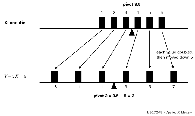
Step 1. Shift and scale. A game pays \({Y = 2X - 5}\) pounds for a die roll \(X\): double the pips and pay 5 to play. Every value is doubled and moved down 5, and so is the balance point.
M06.7.2-F2
\({Y = 2X - 5}\) moves each value of \(X\), keeping its probability. The pivot moves the same way: \({\E[Y] = 2 \times 3.5 - 5 = 2}\).
In symbols, using the rule for \({\E[g(X)]}\) with \({g(x) = ax + b}\):
Step 2. Two variables on one sample space.\(X\) and \(Y\) are both functions of the same outcome \(\omega\). Their sum is the random variable whose value at \(\omega\) is \({X(\omega) + Y(\omega)}\): one column of the anchor picture. The last lesson showed that an expectation can be taken over the outcomes, \({\E[X]}\)\({= \sum_\omega X(\omega)\,\Prob(\{\omega\})}\). That is the tool for sums.
Step 3. Counts as sums of indicators. The number of heads in \(n\) flips is \({I_1 + I_2 + \dots + I_n}\), where \(I_k\) is the indicator of a head on flip \(k\). Each indicator has expectation \({\Prob(\text{head}) = 1/2}\) (M06.7.1). If expectations add, the expected number of heads is \({n/2}\), without ever writing down the binomial PMF.
The formal statement
NoteLinearity of expectation
For any random variables \(X\) and \(Y\) on the same sample space, with finite expectations, and any numbers \(a\) and \(b\), \[
\E[aX + b] = a\,\E[X] + b,
\]\[
\E[X + Y] = \E[X] + \E[Y].
\] By repeating the second rule, \({\E[X_1 + \dots + X_n]}\)\({= \E[X_1] + \dots + \E[X_n]}\). No independence is assumed.
Proof of the sum rule (discrete sample space). Sum over the outcomes and split the sum:
Each outcome is used once with its own probability. How \(X\) and \(Y\) depend on each other never enters. For densities the same steps work with integrals.
Products need independence. For independent \(X\) and \(Y\), \({\E[XY] = \E[X]\,\E[Y]}\). Independence of random variables (M06.5.4) says \({\Prob(X = x, Y = y)}\)\({= p_X(x)\,p_Y(y)}\). The product \(XY\) is a function of the pair, so by the rule for functions, applied to the pair:
The third line takes the factor that does not depend on \(y\) out of the inner sum.
M06.7.2-F3
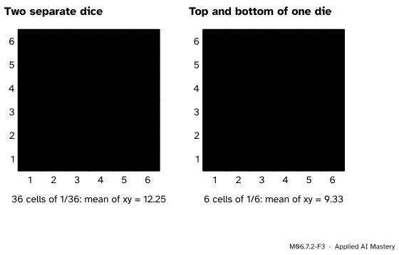
Where the weight sits on the dice grid. Two separate dice spread it over all 36 pairs, and the mean of \({xy}\) is \({3.5 \times 3.5 = 12.25}\). The top and bottom faces of one die always add to 7, so all the weight sits on six cells and the mean of \({xy}\) falls to \({28/3 \approx 9.33}\).
For the top face \(X\) and the bottom face \({Y = 7 - X}\) of one die, \(Y\) is fixed by \(X\):
not 12.25. (The six products are \({1 \cdot 6}\), \({2 \cdot 5}\), and so on.)
Yet \({X + Y = 7}\) on every roll, so \({\E[X + Y] = 7 = 3.5 + 3.5}\): the sum rule holds even for this pair, which is as dependent as two variables can be.
Worked example
Heads in \(n\) flips. With \({I_k}\) the indicator of a head on flip \(k\),
For 10 flips, 5 heads on average. The same argument gives the expected number of correct answers on a test set of \(n\) examples, each correct with probability 0.9: \({0.9\,n}\).
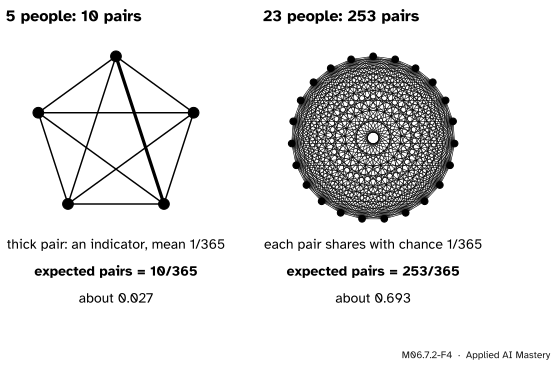
Shared birthdays among 23 people. Ignore leap years and assume all 365 birthdays are equally likely and independent between people. For each pair of people \(\{i, j\}\), let \(I_{ij}\) be the indicator that they share a birthday. Whatever \(i\)’s birthday is, \(j\) matches it with probability \(1/365\), so \({\E[I_{ij}] = 1/365}\). The number of shared pairs is the sum of the \(I_{ij}\) over all pairs, and there are \({\binom{23}{2}}\)\({= 23 \cdot 22/2}\)\({= 253}\) pairs. So
One indicator per pair. Five people make 10 pairs; 23 people make 253. Each pair contributes \(1/365\) to the expected count, so the total is the number of pairs over 365.
The indicators overlap: if Ann matches Ben and Ben matches Cal, then Ann matches Cal. That would matter for the full distribution of the count, but linearity does not care. (The probability that at least one pair matches is a different number, just over one half at 23 people, from M06.2.2.)
Code
From scratch with exact fractions, then checks by simulation.
from fractions import Fractionfrom itertools import productfrom math import combdie = {k: Fraction(1, 6) for k inrange(1, 7)}E =lambda pmf, g=lambda x: x: sum(g(x) * p for x, p in pmf.items())# Shift and scale, and the sum of X and Y over the eight outcomes of three flips.print("E[2X - 5] =", E(die, lambda x: 2* x -5))flips =list(product("HT", repeat=3))X = [w[:2].count("H") for w in flips]Y = [w[1:].count("H") for w in flips]print("E[X], E[Y], E[X + Y]:", Fraction(sum(X), 8), Fraction(sum(Y), 8), Fraction(sum(X) +sum(Y), 8))# Products: two separate dice against the top and bottom face of one die.two_dice = Fraction(sum(a * b for a, b in product(range(1, 7), repeat=2)), 36)top_bottom = E(die, lambda x: x * (7- x))print("E[XY], separate dice:", two_dice, " top and bottom:", top_bottom)# Indicators: heads in 10 flips, and shared-birthday pairs among 23 people.print("expected heads in 10 flips:", 10* Fraction(1, 2))print("pairs:", comb(23, 2), " expected shared pairs:", comb(23, 2) * Fraction(1, 365))
E[2X - 5] = 2
E[X], E[Y], E[X + Y]: 1 1 2
E[XY], separate dice: 49/4   top and bottom: 28/3
expected heads in 10 flips: 5
pairs: 253   expected shared pairs: 253/365
Now simulate 50,000 rooms of 23 people and count the matching pairs in each. Comparing every person with every person gives a 23 by 23 table of matches per room; it counts each pair twice and each person once against themselves, hence the correction.
import numpy as nprng = np.random.default_rng(23)rooms = rng.integers(0, 365, size=(50_000, 23))matches = rooms[:, :, None] == rooms[:, None, :]pairs = (matches.sum(axis=(1, 2)) -23) //2print("average shared pairs:", pairs.mean().round(3), " exact:", round(253/365, 3))die_a, die_b = rng.integers(1, 7, size=(2, 200_000))print("separate dice, mean of XY:", (die_a * die_b).mean().round(2))print("top and bottom, mean of XY:", (die_a * (7- die_a)).mean().round(2))print("mean of X squared:", (die_a **2).mean().round(2), " square of the mean:", (die_a.mean() **2).round(2))
average shared pairs: 0.694   exact: 0.693
separate dice, mean of XY: 12.26
top and bottom, mean of XY: 9.33
mean of X squared: 15.19   square of the mean: 12.27
The simulated averages land within a few hundredths of the exact answers; the exact digits depend on the seed.
Explore
The balance beam in lesson M06.7.3 has buttons for \({aX + b}\). Press them and check that the pivot moves to \({a\,\E[X] + b}\), whatever shape the bars have.
Pitfalls
M06.7.2-F5
Wrong beside right for \({g(x) = x^2}\) and a die. Squaring the mean gives the curve’s height at 3.5, which is 12.25. The mean of the squares averages the six heights, 15.17, and lies above the curve because the curve bends upwards.
“To find E[g(X)], put E[X] into g.”
Only when \(g\) is a straight line, \({g(x) = ax + b}\). For a curve that bends upwards, such as \(x^2\) or \(e^x\), the average of \(g\) lies above \(g\) of the average (unless \(X\) is a constant): \({\E[X^2] = 91/6}\) but \({(\E[X])^2 = 49/4}\) for a die. Their gap, \({35/12}\), is the variance of the next lesson. In machine learning, the average loss of a model is not the loss at the average input.
“Linearity needs independence.”
The sum rule needs nothing: the anchor’s \(X\) and \(Y\) share a flip, the top and bottom faces of a die are tied completely, and the birthday indicators overlap, yet expectations add in every case. It is the product rule \({\E[XY] = \E[X]\,\E[Y]}\) that needs independence, and the variance of a sum in the next lesson.
“E[X/Y] = E[X]/E[Y].”
Division is not linear either. For the hand density, \({\E[1/X] = 2}\) while \({1/\E[X] = 1.5}\) (exercise 2 of M06.7.1).
Check yourself
Recall
1. State linearity of expectation.
Show answer
\({\E[aX + b] = a\,\E[X] + b}\) and \({\E[X + Y] = \E[X] + \E[Y]}\), for any random variables with finite expectations, dependent or not.
2. Why is no independence needed for the sum rule?
Show answer
Summing \({(X(\omega) + Y(\omega))\,\Prob(\{\omega\})}\) over the outcomes splits into two sums, one for each variable; how they relate never enters.
3. What is the expected number of heads in \(n\) fair flips, and how do indicators give it?
Show answer
\({n/2}\): the count is the sum of \(n\) indicators, each with expectation \(1/2\).
4. When does \({\E[XY] = \E[X]\,\E[Y]}\) hold for sure?
Show answer
When \(X\) and \(Y\) are independent. It can fail otherwise: the top and bottom faces of a die give \({28/3}\), not \({49/4}\).
5. For a die, compare \({\E[X^2]}\) and \({(\E[X])^2}\).
Show answer
\({\E[X^2] = 91/6 \approx 15.17}\) and \({(\E[X])^2 = 49/4 = 12.25}\); the first is larger.
Exercises
1.★ A die roll \(X\) is turned into \({Y = 3X + 2}\). Find \({\E[Y]}\), and the expected total of 4 dice.
Show solution
\({\E[Y]}\)\({= 3 \times 3.5 + 2}\)\({= 12.5}\). The total of 4 dice is a sum of 4 variables each with mean 3.5, so its expectation is \({4 \times 3.5 = 14}\).
2.★★ Ten letters are put into ten addressed envelopes at random, every order equally likely. What is the expected number of letters in their own envelope?
Show solution
Let \(I_k\) be the indicator that letter \(k\) lands in envelope \(k\). In a random order letter \(k\) is equally likely to be in any of the ten envelopes, so \({\E[I_k] = 1/10}\). The count is \({I_1 + \dots + I_{10}}\), so its expectation is \({10 \times 1/10 = 1}\). The indicators are dependent (if nine letters are right, so is the tenth), and it does not matter.
3.★★★ Flip a fair coin 10 times. What is the expected number of places where a head is immediately followed by another head? (In HHHT there are two such places.)
Show solution
There are 9 neighbouring pairs of flips, positions \({(1, 2), \dots, (9, 10)}\). Let \(J_k\) be the indicator that flips \(k\) and \({k + 1}\) are both heads; \({\E[J_k]}\)\({= \tfrac12 \cdot \tfrac12}\)\({= \tfrac14}\). The count is \({J_1 + \dots + J_9}\), so its expectation is \({9/4 = 2.25}\). Neighbouring indicators share a flip and are dependent, and linearity still applies.
Summary card
Expectations add, whatever the dependence.
M06.7.2-F1
Average of the stacks = sum of the averages.
\({\E[aX + b] = a\,\E[X] + b}\) and \({\E[X + Y] = \E[X] + \E[Y]}\), no independence needed.
Indicators: a count is a sum of indicators, so its mean is a sum of probabilities.
Products:\({\E[XY] = \E[X]\,\E[Y]}\) when \(X\) and \(Y\) are independent.
Curves:\({\E[g(X)] \neq g(\E[X])}\) unless \(g\) is a straight line.
Sources and next steps
Sources. Each was opened and checked against this lesson on 14 November 2026.
Jeremy Orloff and Jonathan Bloom, Reading 4b: Discrete Random Variables: Expected Value, MIT OpenCourseWare 18.05, Spring 2022. Section 2.2 states \({\E[X + Y] = \E[X] + \E[Y]}\) and \({\E[aX + b] = a\E[X] + b}\); Section 2.4 proves the sum rule with a table of outcomes, as here; Section 2.3 warns that \({\E[h(X)] = h(\E[X])}\) is not true in general.
Charles M. Grinstead and J. Laurie Snell, Introduction to Probability, second edition, Section 6.1: Theorem 6.2 (expectations of sums and multiples) and Theorem 6.4 (\({\E(X \cdot Y) = \E(X)\E(Y)}\) for independent variables), with its proof by factoring the double sum.
Hossein Pishro-Nik, Expectation, Introduction to Probability, Statistics, and Random Processes, Section 3.2.2: the theorem on linearity, for any set of random variables.
Chris Piech, Expectation, Probability for Computer Scientists: the sum rule holds whether or not the variables are dependent, and the rule for \({\E[g(X)]}\) appears under the name LOTUS.