Ratings, grades and severity levels come in an order. The proportional-odds model cuts one score with increasing thresholds; its likelihood is derived and maximised from scratch on the diabetes data in four grades, beside the Frank and Hall reduction and metrics that respect the order.
ML02.10.4L2 Intermediate25 minIn review (what this means)
The maths and code on this page are checked by automated tests on every change, but an independent reader has not signed it off yet. Spot a mistake or a confusing step? Tell us.
Explain what plain multi-class classification and plain regression each get wrong about ordered classes.
State the proportional-odds model, derive its grade probabilities and its likelihood, and fit it with scipy.optimize.minimize.
Build the Frank and Hall reduction to K - 1 binary questions and combine its answers into grade probabilities.
Compute the mean absolute error on grade numbers and the quadratic weighted kappa, and say why they suit ordered classes.
The question
A model reads a patient’s record and predicts the severity of their disease on a scale of 1 to 4. The true grade is 1. Predicting 2 is a small slip; predicting 4 could send a healthy person to intensive care. Accuracy calls both “wrong”. How do we build a model, and a score, that know 4 is further from 1 than 2 is?
From the last lesson
1. Define the Hamming loss of a multi-label prediction.
Show answer
The share of the \(nL\) cells of the label matrix that are predicted wrong.
2. What does a classifier chain give classifier \(j\) that binary relevance does not?
Show answer
The labels before it in the chain: true labels during training, the chain’s own predictions at prediction time.
Intuition
Ordered classes, called ordinal, sit between two tools we already have, and both fit badly. Multi-class classification (lesson 1) treats the grades as unordered names: swap the labels 2 and 4 and it learns the same model. Regression on the numbers 1 to 4 keeps the order but assumes the steps are equal, so that 1 to 2 is the same distance as 3 to 4, which nothing guarantees for “mild, moderate, severe, critical”.
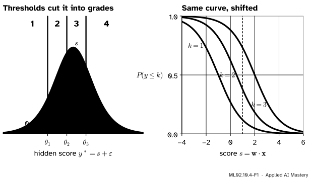
The cumulative-link model keeps the order and nothing more. It computes a single score \({s = \vect{w} \cdot \vect{x}}\) and cuts the score line at increasing thresholds\({\theta_1 < \theta_2 < \theta_3}\).
ML02.10.4-F1
The proportional-odds model with thresholds \({(-1,\ 0.5,\ 2)}\). Left: the score plus random noise lands in one of four bands; each band’s area is the probability of that grade. Right: the chance of a grade of at most \(k\) is the same S-shaped curve for every \(k\), shifted by its threshold.
Read the left panel as a story. The example has a hidden severity \({y^* = s + \varepsilon}\), its score plus noise. The grade we see is the band that \(y^*\) falls in. A higher score pushes the whole bump to the right, making high grades more likely, and the order of the grades is built into the order of the bands.
Build it up
Step 1. The hidden score.\({y^* = s + \varepsilon}\), where \(\varepsilon\) has the logistic distribution, whose cumulative distribution function is the sigmoid \(\sigma\) of ML01.6.1.
Step 2. Cumulative probabilities. The grade is at most \(k\) exactly when \({y^* \le \theta_k}\):
Step 3. Grade probabilities. Grade \(k\) is “at most \(k\), but not at most \({k - 1}\)”, so its probability is the gap between two neighbouring cumulative curves:
with the conventions \({\theta_0 = -\infty}\) and \({\theta_K = +\infty}\), so that \({\sigma(-\infty) = 0}\) and \({\sigma(+\infty) = 1}\).
Step 4. Why the thresholds must increase.\(\sigma\) is increasing, so every gap is positive exactly when \({\theta_{k-1} < \theta_k}\). Out-of-order thresholds would give negative probabilities.
ML02.10.4-F2
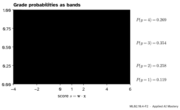
The four grade probabilities stacked. As the score grows, the probability flows from grade 1 to grade 4 through the grades in between, never skipping one.
The formal statement
NoteThe proportional-odds model
For ordered grades \({1, \dots, K}\), weights \(\vect{w}\) and thresholds \({\theta_1 < \dots < \theta_{K-1}}\),
It has \(d\) weights and \({K - 1}\) thresholds. The weights have no separate bias, because a bias would only shift every threshold by the same amount.
Why “proportional odds”. Take the log-odds of the event \({y \le k}\). Since \({\ln\frac{\sigma(z)}{1 - \sigma(z)} = z}\) (ML01.6.1),
\[
\ln \frac{\Prob(y \le k \mid \vect{x})}{\Prob(y > k \mid \vect{x})} = \theta_k - \vect{w} \cdot \vect{x} .
\]
Compare two inputs \(\vect{x}\) and \(\vect{x}'\). The difference of their log-odds is \({-\vect{w} \cdot (\vect{x} - \vect{x}')}\): the threshold cancels. So the ratio of the odds is the same for every cut \(k\); the odds are proportional. One weight vector serves all \({K - 1}\) cuts, against \({(K - 1)(d + 1)}\) parameters for softmax regression with a baseline class.
The likelihood. For \(n\) independent examples with grades \(y_i\) and scores \({s_i = \vect{w} \cdot \vect{x}_i}\), the likelihood is the product of the probabilities of the grades that were observed. Its negative logarithm, to be minimised, is
For \({K = 2}\) there is one threshold, and the bracket is \({\sigma(\theta_1 - s_i)}\) for grade 1 and \({1 - \sigma(\theta_1 - s_i)}\) for grade 2: the log loss of ML01.6.2 with score \({s_i - \theta_1}\).
Keeping the thresholds in order. A general-purpose optimiser does not know about the constraint \({\theta_1 < \theta_2 < \dots}\). Write the thresholds through free numbers \(a_1, \dots, a_{K-1}\):
Every gap \(e^{a_k}\) is positive, so any \(\vect{a}\) gives ordered thresholds, and minimize can search freely over \(\vect{w}\) and \(\vect{a}\).
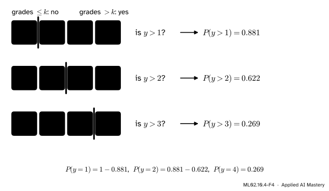
The Frank and Hall reduction. Ask \({K - 1}\) binary questions “is \({y > k}\)?”, each answered by its own binary classifier with a probability \({q_k = \Prob(y > k)}\). Then
and the grade with the largest probability is predicted. Any classifier that outputs probabilities can be used, a tree as well as logistic regression.
ML02.10.4-F4
Four ordered grades become three yes-or-no questions. The differences of their answers give the grade probabilities.
With logistic regression for each question, Frank and Hall is the proportional-odds model with the shared weight vector cut loose: every question gets its own \(\vect{w}_k\). That is more flexible, but the separately fitted curves can cross, and then a difference such as \({\Prob(y > 1) - \Prob(y > 2)}\) comes out negative.
Metrics that respect the order. The mean absolute error on the grade numbers (ML01.7.4) charges a miss by its distance. The quadratic weighted kappa compares the confusion matrix \(O\) with the matrix \(E\) expected by chance, charging each cell \({(i - j)^2}\). If row \(i\) of \(O\) adds up to \(r_i\) and column \(j\) to \(c_j\), then \({E_{ij} = r_i c_j / n}\), and
\[
\kappa_w = 1 - \frac{\sum_{i,j} (i - j)^2\, O_{ij}}{\sum_{i,j} (i - j)^2\, E_{ij}} .
\]
It is 1 for perfect agreement, about 0 for predictions no better than chance, and negative for worse.
Worked example
One example by hand. Thresholds \({\vect{\theta} = (-1,\ 0.5,\ 2)}\) and score \({s = 1}\).
ML02.10.4-F3
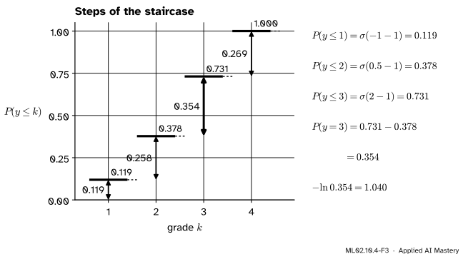
The cumulative probabilities form a staircase; each step’s height is a grade probability.
The cumulative probabilities are \({\sigma(-2) = 0.119}\), \({\sigma(-0.5) = 0.378}\) and \({\sigma(1) = 0.731}\). The grade probabilities are the steps:
They add up to 1, and grade 3 is the most likely. If the true grade is 3, this example adds \({-\ln 0.354 = 1.040}\) to the negative log-likelihood. (The steps use unrounded values, so \({0.378 - 0.119}\) prints as \(0.258\).) The Frank and Hall figure uses the same example: \({\Prob(y > k) = 1 - \Prob(y \le k)}\) gives \(0.881\), \(0.622\) and \(0.269\).
A weighted kappa by hand. Ten examples with true grades \({(1, 1, 2, 2, 2, 3, 3, 3, 4, 4)}\). Model A predicts \({(1, 2, 2, 1, 2, 3, 4, 3, 4, 3)}\): six right and four misses, each by one grade. Its accuracy is \(0.6\), its MAE \({4/10 = 0.4}\), and \({\sum (i - j)^2 O_{ij} = 4}\).
For \(E\), the true grades have counts \({(2, 3, 3, 2)}\) and model A’s predictions too. Group the cells by distance: six cells at distance 1 with \({r_i c_j}\) summing to 42, four at distance 2 summing to 24, and two at distance 3 summing to 8. Weighted by 1, 4 and 9 these give \(42\), \({4 \cdot 24 = 96}\) and \({9 \cdot 8 = 72}\), so
The diabetes data of ML01.10, with its target, a measure of disease progression, cut at 90, 140 and 210 into four ordered grades. First the negative log-likelihood and its minimisation, from scratch.
Body mass index (bmi) and the serum measure s5 push the grade up most. The large negative weight on s1 sits beside a positive one on s2, two strongly correlated blood measures, so read those two with care (ML01.9).
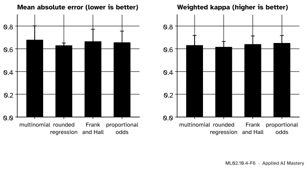
Now four ways to predict the grades, compared by 5-fold cross-validation on the order-aware metrics. The kappa is computed from scratch once and checked against scikit-learn.
from sklearn.linear_model import LinearRegression, LogisticRegressionfrom sklearn.metrics import cohen_kappa_score, confusion_matrix, mean_absolute_errorfrom sklearn.model_selection import KFolddef qwk(y_true, y_pred, K=4): O = confusion_matrix(y_true, y_pred, labels=range(1, K +1)) E = np.outer(O.sum(axis=1), O.sum(axis=0)) / O.sum() i, j = np.indices((K, K))return1- ((i - j) **2* O).sum() / ((i - j) **2* E).sum()def grade_probs(X, w, theta): cum = expit(theta[None, :] - (X @ w)[:, None])return np.diff(np.c_[np.zeros(len(X)), cum, np.ones(len(X))], axis=1)raw = data.datascores = {name: [] for name in ("multinomial", "regression", "Frank-Hall", "ordinal")}for train, test in KFold(5, shuffle=True, random_state=0).split(raw): scaler = StandardScaler().fit(raw[train]) A, B, ya, yb = scaler.transform(raw[train]), scaler.transform(raw[test]), y[train], y[test] wf, thf = unpack(minimize(nll, np.r_[np.zeros(d), -1, 0, 0], args=(A, ya), method="BFGS").x) G = np.column_stack([LogisticRegression().fit(A, ya > k).predict_proba(B)[:, 1] for k in (1, 2, 3)]) F = np.c_[1- G[:, 0], G[:, 0] - G[:, 1], G[:, 1] - G[:, 2], G[:, 2]] preds = {"multinomial": LogisticRegression().fit(A, ya).predict(B),"regression": np.clip(np.rint(LinearRegression().fit(A, ya).predict(B)), 1, 4).astype(int),"Frank-Hall": F.argmax(axis=1) +1,"ordinal": grade_probs(B, wf, thf).argmax(axis=1) +1}for name, p in preds.items():assert np.isclose(qwk(yb, p), cohen_kappa_score(yb, p, weights="quadratic")) scores[name].append((mean_absolute_error(yb, p), qwk(yb, p)))for name, s in scores.items(): s = np.array(s)print(f"{name:>11}: MAE {s[:, 0].mean():.3f} (sd {s[:, 0].std():.3f}) kappa {s[:, 1].mean():.3f}"f" (sd {s[:, 1].std():.3f})")
multinomial: MAE 0.676 (sd 0.126)   kappa 0.629 (sd 0.089)
 regression: MAE 0.627 (sd 0.024)   kappa 0.613 (sd 0.052)
 Frank-Hall: MAE 0.662 (sd 0.109)   kappa 0.637 (sd 0.076)
    ordinal: MAE 0.653 (sd 0.102)   kappa 0.648 (sd 0.069)
ML02.10.4-F6
Cross-validated scores on the four diabetes grades. The ordinal model has the highest kappa and a lower error than softmax regression; rounded regression has the lowest error. The whiskers are wider than the gaps.
Read the result honestly. The proportional-odds model, with 13 parameters, beats softmax regression, with 33, on both order-aware metrics. Rounded regression wins on mean absolute error but has the lowest kappa. And the differences are smaller than the spread from fold to fold, so this dataset does not separate the methods; lesson ML02.11.3 shows how to compare models fairly.
Explore
This module’s interactive, the reduction explorer, is in lesson ML02.10.2. Its softmax mode shows the multi-class model that this lesson improves on for ordered classes: three free score vectors, where the proportional-odds model would use one.
Pitfalls
ML02.10.4-F5
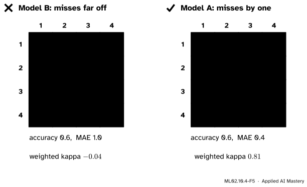
Wrong beside right. Both models have accuracy \(0.6\). Model B’s misses are two or three grades off, model A’s only one; the mean absolute error and the weighted kappa see the difference.
“Accuracy is fine for grades.”
Accuracy, and the unweighted kappa too, count every miss the same. For the two models in the figure the unweighted kappa even prefers model B, \(0.474\) against \(0.459\). Use a distance-aware score: the MAE on grade numbers, or the quadratic weighted kappa.
“Ordinal means I can just regress on 1, 2, 3, 4.”
Regression assumes the grades are equally spaced and that a prediction of \(2.5\) means something. The proportional-odds model learns the spacing from the data instead: on the diabetes grades its thresholds are \({-1.66}\), \({-0.13}\) and \({1.66}\), with gaps of \(1.53\) and \(1.79\), and it gives a probability for each grade rather than a number between grades.
“Frank and Hall always gives valid probabilities.”
Its \({K - 1}\) classifiers are fitted separately, so nothing stops \({\Prob(y > 2)}\) from exceeding \({\Prob(y > 1)}\) for some input, and then \({\Prob(y = 2)}\) comes out negative. The cumulative-link model cannot do this: one score and ordered thresholds keep its cumulative curves in order.
Check yourself
Recall
1. What does multi-class classification ignore about ordered classes, and what does regression assume?
Show answer
Multi-class ignores the order: relabelling the grades changes nothing. Regression assumes the grades are equally spaced numbers.
2. Write the cumulative probability of the proportional-odds model.
Show answer
\({\Prob(y \le k \mid \vect{x}) = \sigma(\theta_k - \vect{w} \cdot \vect{x})}\), with increasing thresholds \({\theta_1 < \dots < \theta_{K-1}}\).
3. How is the probability of grade \(k\) obtained from the cumulative probabilities?
Show answer
As the difference \({\sigma(\theta_k - s) - \sigma(\theta_{k-1} - s)}\), with \({\theta_0 = -\infty}\) and \({\theta_K = +\infty}\).
4. What are the binary questions of the Frank and Hall reduction?
Show answer
“Is \({y > k}\)?” for \({k = 1, \dots, K - 1}\), one classifier each.
5. What does the quadratic weighted kappa charge for a miss from grade \(i\) to grade \(j\)?
Show answer
\({(i - j)^2}\), measured against the same charge on the table expected by chance.
Exercises
1.★ Thresholds \({(-1,\ 0.5,\ 2)}\) and score \({s = 3}\). Find the four grade probabilities and the most likely grade.
Show solution
\({\sigma(-4) = 0.018}\), \({\sigma(-2.5) = 0.076}\), \({\sigma(-1) = 0.269}\). The grade probabilities are \(0.018\), \({0.076 - 0.018 = 0.058}\), \({0.269 - 0.076 = 0.193}\) and \({1 - 0.269 = 0.731}\). Grade 4 is the most likely.
2.★★ Show that in the proportional-odds model the odds of \({y \le k}\) for input \(\vect{x}\), divided by the odds for \(\vect{x}'\), equal \({e^{-\vect{w}\cdot(\vect{x} - \vect{x}')}}\) for every \(k\). What happens to the odds of a low grade when the score rises by 1?
Show solution
The odds of \({y \le k}\) are \({\sigma(z)/(1 - \sigma(z)) = e^{z}}\) with \({z = \theta_k - \vect{w}\cdot\vect{x}}\). Dividing,
\(\theta_k\) cancels, so the ratio is the same for every \(k\). When the score rises by 1, the odds of “grade \(k\) or lower” are multiplied by \({e^{-1} = 0.368}\), for every \(k\) at once.
3.★★★ Compute the mean absolute error and the quadratic weighted kappa of model B in the pitfall figure: true grades \({(1, 1, 2, 2, 2, 3, 3, 3, 4, 4)}\), predictions \({(1, 4, 2, 4, 2, 3, 1, 3, 4, 1)}\).
Show solution
The misses are \({1 \to 4}\), \({2 \to 4}\), \({3 \to 1}\) and \({4 \to 1}\), at distances 3, 2, 2 and 3, so the MAE is \({10/10 = 1.0}\), and \({\sum (i - j)^2 O_{ij}}\)\({= 9 + 4 + 4 + 9}\)\({= 26}\). The row totals are \({(2, 3, 3, 2)}\) and the prediction counts \({(3, 2, 2, 3)}\). Group the products \({r_i c_j}\) by distance:
Weighted by 1, 4 and 9 these give \(38\), \({104}\) and \({108}\), which add up to \(250\), so \({\sum (i - j)^2 E_{ij}}\)\({= 250/10 = 25}\), and \({\kappa_w = 1 - 26/25 = -0.04}\): worse than chance.
Summary card
One score, increasing thresholds: the order of the grades is built into the model.
ML02.10.4-F1
Thresholds cut one score into grades.
Model.\({\Prob(y \le k \mid \vect{x})}\)\({= \sigma(\theta_k - \vect{w}\cdot\vect{x})}\), with \({\theta_1 < \dots < \theta_{K-1}}\).
Fit. Minimise \({-\sum_i \ln \Prob(y_i \mid \vect{x}_i)}\), with \({\theta_k = \theta_{k-1} + e^{a_k}}\).
Frank and Hall.\({K - 1}\) questions “\({y > k}\)?”, combined by differences.
Metrics. MAE on grade numbers; \({\kappa_w}\) with weights \({(i - j)^2}\).
Sources and next steps
Sources. Each was opened and checked against this lesson on 15 November 2026.
R documentation for MASS::polr, ordered logistic or probit regression: the model \({\operatorname{logit} P(Y \le k \mid x) = \zeta_k - \eta}\) with increasing cut points \(\zeta\) and a linear predictor \(\eta\) without intercept, and the name proportional odds, because the log odds of the different categories differ only by a constant.
Eibe Frank and Mark Hall, A Simple Approach to Ordinal Classification, University of Waikato working paper 01/5, 2001, also published at ECML 2001. Section 2: the \(k\)-class ordinal problem turned into \({k - 1}\) binary problems “Target > \(V_i\)”, the formulas for \({\Pr(V_1)}\), \({\Pr(V_i)}\) and \({\Pr(V_k)}\) as differences, and prediction by the largest probability.
scikit-learn 1.9, cohen_kappa_score: kappa as observed against chance agreement, with weights="linear" or "quadratic". The weighted formula in this lesson was checked numerically against it in the code above.
Next. Module ML02.11, Choosing a model for tabular data, puts the models of this course side by side and compares them fairly.