Ask which direction best separates the classes, with no Gaussians at all: maximise the spread between the projected class means over the spread within. Derive Fisher’s direction, find that it is LDA’s, and use the K - 1 discriminant directions to draw wine in two dimensions beside PCA.
ML02.9.4L2 Intermediate25 minIn review (what this means)
The maths and code on this page are checked by automated tests on every change, but an independent reader has not signed it off yet. Spot a mistake or a confusing step? Tell us.
State Fisher’s criterion, the ratio of between-class to within-class scatter along a direction, and compute it for a given direction.
Derive that for two classes the best direction is proportional to the inverse within-class scatter times the difference of the means, the same direction as LDA.
Set up the K-class problem as a generalised eigenproblem and explain why it has at most K - 1 useful directions.
Project a data set onto its discriminant directions and contrast the result with principal components.
The question
In a 1936 paper on measurements of iris flowers, R. A. Fisher asked a question that needs no bell curves at all: if we may look at the data along one direction only, which direction shows the classes most clearly apart? And with three or more classes, what is the best flat picture of them?
From the last lesson
1. How many covariance parameters do LDA and QDA estimate?
Show answer
LDA \({d(d + 1)/2}\); QDA \({K\,d(d + 1)/2}\).
2. Why is the covariance of a class with \({n_k \le d}\) points singular?
Show answer
Its deviations from the class mean sum to zero, so they span at most \({n_k - 1 < d}\) directions.
Intuition
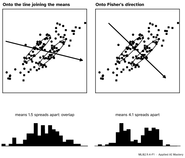
Projecting onto a direction turns each point into one number, and each class into a pile of numbers. Good separation means two piles whose centres are far apart compared with how wide the piles are. The obvious choice, the line through the two class means, puts the centres far apart, but if the clouds are long and tilted it also makes the piles wide.
ML02.9.4-F1
The same two classes projected two ways. Along the line joining the means the piles overlap. Along Fisher’s direction, which cuts across the clouds’ length, they separate.
Fisher’s direction trades a little distance between the centres for a lot less width. It looks across the clouds’ thin side, where each class is narrow, rather than along their length.
Build it up
Step 1. Project. For a direction \(\vect{w}\), a point becomes the number \({z = \vect{w}\T\vect{x}}\). The class means become \({\vect{w}\T\vect{\mu}_0}\) and \({\vect{w}\T\vect{\mu}_1}\), so they are \({\vect{w}\T(\vect{\mu}_1 - \vect{\mu}_0)}\) apart.
Step 2. Measure the width of the piles. The projected scatter of class \(k\) about its own projected mean is
where \({\vect{v}_i = \vect{x}_i - \vect{\mu}_k}\). The middle step uses \({(\vect{w}\T\vect{v})^2 = \vect{w}\T\vect{v}\,\vect{v}\T\vect{w}}\), true for any vector \(\vect{v}\). Adding over the classes gives \({\vect{w}\T\mat{S}_W\vect{w}}\), with \(\mat{S}_W\) the within-class scatter matrix of ML02.9.2.
Step 3. Take the ratio. Fisher’s criterion is the squared distance between the projected means over the total projected scatter. Doubling \(\vect{w}\) multiplies the top and the bottom by four, so only the direction matters.
ML02.9.4-F2
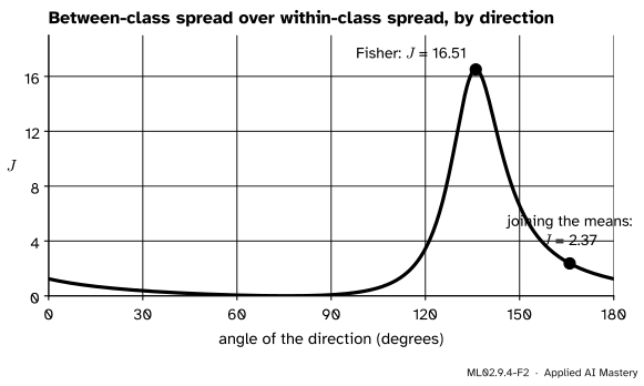
Fisher’s ratio for every direction through the tilted clouds. The spread within is measured per point, with the clouds’ covariance \(\mat{\Sigma}\) in place of \(\mat{S}_W\); that multiplies every \(J\) by the same number and does not move the peak. The direction joining the means scores 2.37; the best direction scores 16.51, seven times as much.
The formal statement
NoteDefinition: Fisher’s criterion
For two classes with means \(\vect{\mu}_0\), \(\vect{\mu}_1\) and within-class scatter matrix \({\mat{S}_W = \sum_k\sum_{i:\,y_i = k}(\vect{x}_i - \vect{\mu}_k)(\vect{x}_i - \vect{\mu}_k)\T}\), Fisher’s criterion for a direction \({\vect{w} \ne \vect{0}}\) is
Fisher’s linear discriminant is the direction that maximises \(J\).
Result: \({\vect{w} \propto \mat{S}_W^{-1}(\vect{\mu}_1 - \vect{\mu}_0)}\). Write \({\vect{d} = \vect{\mu}_1 - \vect{\mu}_0}\). \(\mat{S}_W\) is symmetric and positive definite, so it has a symmetric square root \(\mat{S}_W^{1/2}\) (take the square roots of its eigenvalues, M03.3). Put \({\vect{v} = \mat{S}_W^{1/2}\vect{w}}\) and \({\vect{a} = \mat{S}_W^{-1/2}\vect{d}}\). Then \({\vect{w}\T\mat{S}_W\vect{w} = \vect{v}\T\vect{v}}\) and \({\vect{w}\T\vect{d} = \vect{v}\T\vect{a}}\), so
by the Cauchy-Schwarz inequality, with equality exactly when \(\vect{v}\) is a multiple of \(\vect{a}\). Undoing the substitution, \({\vect{w} = \mat{S}_W^{-1/2}\vect{v} \propto \mat{S}_W^{-1/2}\vect{a} = \mat{S}_W^{-1}\vect{d}}\), and the best value is \({\norm{\vect{a}}^2 = \vect{d}\T\mat{S}_W^{-1}\vect{d}}\).
It is LDA’s direction. The pooled covariance of ML02.9.2 is \({\hat{\mat{\Sigma}} = \mat{S}_W/n}\), so \({\hat{\mat{\Sigma}}^{-1}\vect{d} = n\,\mat{S}_W^{-1}\vect{d}}\): the same direction. Fisher assumed nothing about Gaussians; he asked only about means and scatters. Gaussian clouds with a shared covariance are what make the cut on that direction, and the posterior probabilities, optimal.
Many classes. With \(K\) classes and overall mean \(\vect{\mu}\), the spread of the class means is the between-class scatter matrix
and Fisher’s criterion becomes \({J(\vect{w}) = \vect{w}\T\mat{S}_B\vect{w} / \vect{w}\T\mat{S}_W\vect{w}}\). (For two classes \({\mat{S}_B = \tfrac{n_0n_1}{n}\vect{d}\vect{d}\T}\), which gives back the criterion above up to a constant factor.) The same substitution gives
a Rayleigh quotient of a symmetric matrix (M03.3.4). Its maximum is the largest eigenvalue of \(\mat{M}\), at its top eigenvector. Multiplying \({\mat{M}\vect{v} = \lambda\vect{v}}\) on the left by \(\mat{S}_W^{-1/2}\) and writing \({\vect{w} = \mat{S}_W^{-1/2}\vect{v}}\) turns it into the generalised eigenproblem
The next best directions are the next eigenvectors; their eigenvalues are their values of \(J\). These are the discriminant directions (ESL calls them canonical variates).
At most \({K - 1}\) of them.\(\mat{S}_B\) is a sum of \(K\) outer products, but the vectors \({\vect{\mu}_k - \vect{\mu}}\) are tied by one equation, \({\sum_k n_k(\vect{\mu}_k - \vect{\mu}) = \vect{0}}\), because \(\vect{\mu}\) is the weighted average of the class means. So they span at most \({K - 1}\) dimensions, \(\mat{S}_B\) has rank at most \({K - 1}\), and so does \({\mat{S}_W^{-1}\mat{S}_B}\): every other eigenvalue is zero. In plain words, \(K\) points (the class means) always lie in a flat space of dimension \({K - 1}\), and nothing outside it helps tell the classes apart.
ML02.9.4-F6
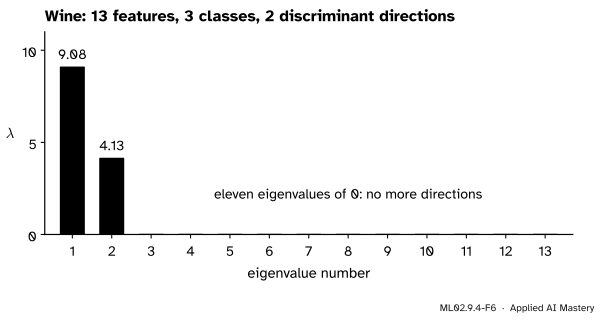
Wine has 13 features but only 3 classes, so Fisher’s eigenproblem has just two non-zero eigenvalues.
Worked example
Find Fisher’s direction for the twelve points, its ratio, and the cut on it.
From ML02.9.2, \({\vect{d} = (2, 1)}\) and \({\mat{S}_W = \tfrac13\begin{bmatrix}62 & 23\\ 23 & 74\end{bmatrix}}\). Its inverse is \({\tfrac{3}{4059}\begin{bmatrix}74 & -23\\ -23 & 62\end{bmatrix}}\), so
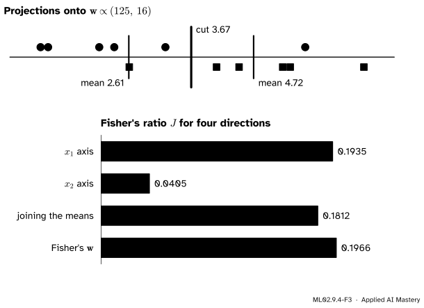
Compare three other directions. Along the \(x_1\) axis, \({J = 2^2/(62/3) = 6/31 = 0.1935}\). Along the \(x_2\) axis, \({J = 1/(74/3) = 3/74 = 0.0405}\). Along the line joining the means,
The worked example. Projected onto Fisher’s direction the classes are piles of numbers with means 2.61 and 4.72; LDA’s cut sits halfway, at 3.67. Below, Fisher’s direction beats the axes and the line joining the means.
Here the clouds are not very elongated across the classes’ separation, so Fisher’s direction is only slightly better than the \(x_1\) axis; for the tilted clouds of the anchor figure it was seven times better than the line joining the means. With unit vector \({\vect{u} = (125, 16)/126.02}\) the projected means are 2.611 and 4.721, and the cut halfway between them is \({462/126.02 = 3.666}\): exactly LDA’s line, seen end on.
Code
Fisher’s direction from scratch on the twelve points, then the many-class version on wine.
import numpy as npfrom scipy.linalg import eighX = np.array([(1, 1), (2, 1), (1, 2), (2, 3), (3, 2), (5, 5), (4, 1), (5, 2), (5, 3), (4, 4), (2, 5), (6, 5)], dtype=float)y = np.array([0] *6+ [1] *6)def scatter_matrices(X, y): mu = X.mean(axis=0) S_W = np.zeros((X.shape[1], X.shape[1])) S_B = np.zeros_like(S_W)for k in np.unique(y): Xk = X[y == k] mk = Xk.mean(axis=0) S_W += (Xk - mk).T @ (Xk - mk) S_B +=len(Xk) * np.outer(mk - mu, mk - mu)return S_W, S_BS_W, S_B = scatter_matrices(X, y)d = X[y ==1].mean(axis=0) - X[y ==0].mean(axis=0)J =lambda w: (w @ d) **2/ (w @ S_W @ w)w = np.linalg.solve(S_W, d)print("Fisher direction, scaled:", (w / w[1] *16).round(4))for name, v in (("x1 axis", [1, 0]), ("x2 axis", [0, 1]), ("joining the means", d), ("Fisher", w)):print(f"J along {name}: {J(np.asarray(v, dtype=float)):.4f}")u = w / np.linalg.norm(w)print("projected means:", [round(X[y == k].mean(axis=0) @ u, 3) for k in (0, 1)])
Fisher direction, scaled: [125.  16.]
J along x1 axis: 0.1935
J along x2 axis: 0.0405
J along joining the means: 0.1812
J along Fisher: 0.1966
projected means: [np.float64(2.611), np.float64(4.721)]
For wine, SciPy’s eigh(S_B, S_W) solves the generalised eigenproblem directly. scikit-learn’s LinearDiscriminantAnalysis(n_components=2) finds the same two directions; it may scale them or flip their signs, so we compare the projections by their correlation.
from sklearn.datasets import load_winefrom sklearn.decomposition import PCAfrom sklearn.discriminant_analysis import LinearDiscriminantAnalysisfrom sklearn.preprocessing import StandardScalerXw, yw = load_wine(return_X_y=True)Z = StandardScaler().fit_transform(Xw)S_W, S_B = scatter_matrices(Z, yw)lam, V = eigh(S_B, S_W) # increasing orderlam, V = lam[::-1], V[:, ::-1]print("eigenvalues:", lam.round(3))lda = LinearDiscriminantAnalysis(n_components=2).fit(Z, yw)T = lda.transform(Z)print("share of the ratio:", (lam[:2] / lam[:2].sum()).round(4), " scikit-learn:", lda.explained_variance_ratio_.round(4))print("|correlation| with scikit-learn's axes:", [round(abs(np.corrcoef(Z @ V[:, j], T[:, j])[0, 1]), 6) for j in (0, 1)])def fisher_total(T, y): S_W, S_B = scatter_matrices(T, y)return np.trace(np.linalg.solve(S_W, S_B))P = PCA(n_components=2).fit_transform(Z)print(f"Fisher's ratio summed over two axes: discriminant {fisher_total(T, yw):.2f}, principal {fisher_total(P, yw):.2f}")
eigenvalues: [ 9.082  4.128  0.     0.     0.     0.    -0.    -0.    -0.    -0.
 -0.    -0.    -0.   ]
share of the ratio: [0.6875 0.3125]  scikit-learn: [0.6875 0.3125]
|correlation| with scikit-learn's axes: [np.float64(1.0), np.float64(1.0)]
Fisher's ratio summed over two axes: discriminant 13.21, principal 6.96
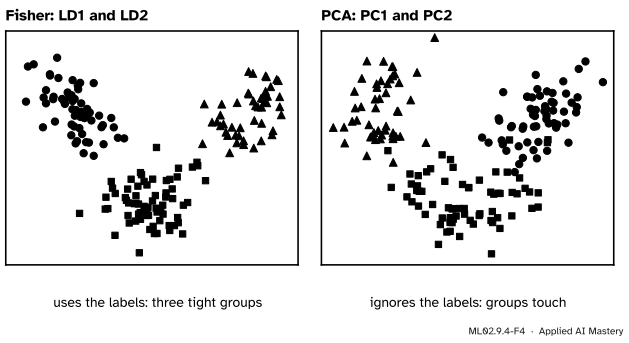
Eleven of the thirteen eigenvalues are zero, as the rank argument promised, and the two non-zero ones split Fisher’s ratio 69% to 31%, which is what scikit-learn reports as explained_variance_ratio_. Asking for n_components=3 raises an error.
ML02.9.4-F4
Wine in two dimensions. Fisher’s directions are chosen to separate the classes; principal components are chosen to keep the most variance and never look at the labels.
The discriminant picture scores 13.21 on Fisher’s ratio summed over its two axes, the principal components 6.96. PCA (M03.6) keeps the directions of greatest total spread, which here happen to separate the wines fairly well too; on other data they need not separate them at all.
Explore
The ellipse explorer of lesson ML02.9.3 draws Fisher’s direction as an orange arrow and the projected classes as histograms beneath the plane. Stretch both ellipses into long cigars side by side and watch the arrow swing across them, then switch the projection to joining the means to see the piles merge.
Pitfalls
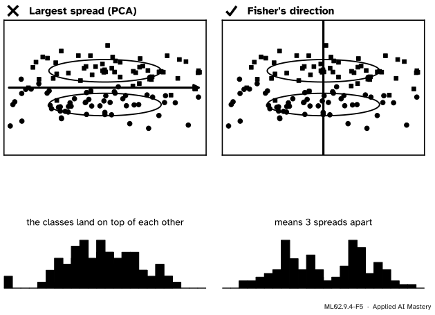
ML02.9.4-F5
Wrong beside right. The direction of largest spread runs along both clouds and separates nothing. Fisher’s direction runs across them.
“The principal components are the directions that best separate the classes.”
PCA never sees the labels. It keeps the directions of greatest spread, and when the classes differ along a direction of small spread, PCA throws exactly that direction away. Use discriminant directions when the aim is separation, principal components when the aim is to keep the data’s shape. ESL’s Figure 4.9 makes the same point with the line joining the centroids.
“LDA can reduce 13 features to any number of components I like.”
To at most \({K - 1}\), here 2, because the between-class scatter has rank at most \({K - 1}\). For two classes LDA gives a single number per example. scikit-learn raises an error if n_components exceeds \({\min(K - 1, d)}\).
“I projected all the data with LDA, then cross-validated a classifier on the projection.”
The projection was fitted with every label, including those of the validation folds, so the validation folds have already influenced the features and the score is optimistic. Fit the projection inside each fold, for example as the first step of a Pipeline (ML04.3 treats this kind of leakage in full).
Check yourself
Recall
1. What does Fisher’s criterion measure for a direction \(\vect{w}\)?
Show answer
The squared distance between the projected class means divided by the total projected within-class scatter: how far apart the piles are compared with how wide they are.
2. What is Fisher’s direction for two classes?
Show answer
\({\vect{w} \propto \mat{S}_W^{-1}(\vect{\mu}_1 - \vect{\mu}_0)}\), the same direction as LDA’s \(\vect{w}\).
3. Which assumption about the data does Fisher’s derivation need?
Show answer
None about their distribution: only class means and scatter matrices. Gaussian classes with a shared covariance are what make the resulting cut optimal.
4. Which eigenproblem gives the discriminant directions for \(K\) classes?
Show answer
\({\mat{S}_B\vect{w} = \lambda\mat{S}_W\vect{w}}\), equivalently the eigenvectors of \({\mat{S}_W^{-1}\mat{S}_B}\), taken in order of decreasing eigenvalue.
5. Why are there at most \({K - 1}\) useful directions?
Show answer
\(\mat{S}_B\) is built from the \(K\) vectors \({\vect{\mu}_k - \vect{\mu}}\), whose weighted sum is zero, so its rank is at most \({K - 1}\) and every other eigenvalue is zero.
Exercises
1.★ Compute Fisher’s ratio for the twelve points along the direction \({(1, 1)}\).
So \({J = 9/(182/3) = 27/182 = 0.148}\), below the 0.1966 of Fisher’s direction.
2.★★ For two classes of sizes \(n_0\) and \(n_1\), show that \({\mat{S}_B = \tfrac{n_0n_1}{n}\vect{d}\vect{d}\T}\) with \({\vect{d} = \vect{\mu}_1 - \vect{\mu}_0}\).
Show solution
The overall mean is \({\vect{\mu} = (n_0\vect{\mu}_0 + n_1\vect{\mu}_1)/n}\). So
For the twelve points that is \({3\,\vect{d}\vect{d}\T}\), as the code checks.
3.★★★ Derive Fisher’s two-class direction a second way, by setting the gradient of \({J(\vect{w}) = (\vect{w}\T\vect{d})^2/(\vect{w}\T\mat{S}_W\vect{w})}\) to zero.
Show solution
Write \({N = (\vect{w}\T\vect{d})^2}\) and \({D = \vect{w}\T\mat{S}_W\vect{w}}\). Their gradients are \({\nabla N = 2(\vect{w}\T\vect{d})\,\vect{d}}\) and \({\nabla D = 2\mat{S}_W\vect{w}}\) (M05.7.1, using that \(\mat{S}_W\) is symmetric). By the quotient rule,
The fraction is a number, so \({\mat{S}_W\vect{w}}\) is a multiple of \(\vect{d}\), and multiplying by \(\mat{S}_W^{-1}\) gives \({\vect{w} \propto \mat{S}_W^{-1}\vect{d}}\).
Summary card
The best direction separates the projected means relative to the spread within the classes, and it is LDA’s.
Two classes:\({\vect{w} \propto \mat{S}_W^{-1}(\vect{\mu}_1 - \vect{\mu}_0)}\), best value \({\vect{d}\T\mat{S}_W^{-1}\vect{d}}\).
\(K\) classes: eigenvectors of \({\mat{S}_W^{-1}\mat{S}_B}\); at most \({K - 1}\) of them.
Versus PCA: uses the labels; PCA keeps spread, Fisher keeps separation.
Sources and next steps
Sources. Each was opened and checked against this lesson on 15 November 2026.
T. Hastie, R. Tibshirani and J. Friedman, The Elements of Statistical Learning, 2nd edition, corrected 12th printing (2017), section 4.3.3: the class centroids lie in an affine subspace of dimension at most \({K - 1}\); Fisher’s problem as the Rayleigh quotient \({\max_a a\T B a / a\T W a}\) (4.15), a generalised eigenvalue problem solved by the largest eigenvalue of \({W^{-1}B}\); the discriminant coordinates, or canonical variates; and Figure 4.9, where the projections onto the line joining the centroids overlap because of the covariance while the discriminant direction separates them.
scikit-learn, Linear and Quadratic Discriminant Analysis, User Guide section 1.2 (dimensionality reduction by projection onto at most \({K - 1}\) dimensions with transform), and the LinearDiscriminantAnalysis reference: n_components must be at most \({\min(K - 1, d)}\), and explained_variance_ratio_.
scikit-learn, The iris plants dataset, section 9.1.1 of the User Guide: the data were first used by R. A. Fisher in “The use of multiple measurements in taxonomic problems”, Annals of Eugenics 7 (1936), 179 to 188.