Give every class the same covariance and the quadratic terms of the log posteriors cancel, leaving a linear boundary. Derive the discriminant line by line, fit it to the twelve points by hand and in NumPy, and compare it with logistic regression.
ML02.9.2L2 Intermediate25 minIn review (what this means)
The maths and code on this page are checked by automated tests on every change, but an independent reader has not signed it off yet. Spot a mistake or a confusing step? Tell us.
Derive the linear discriminant function from the Gaussian log posterior with a shared covariance, showing why the quadratic term cancels.
Estimate the pooled within-class covariance and compute the LDA boundary of a small data set by hand.
Show that the log-odds of two-class LDA are linear in the features, and say how LDA and logistic regression differ in the way they fit that form.
Explain when LDA tends to beat logistic regression and when logistic regression is the safer choice.
The question
Each class of the twelve points is a tilted cloud. Suppose we insist that all classes share one shape, the same covariance matrix, and differ only in where they sit. What does the boundary between them become, and why would anyone accept such a strong assumption?
From the last lesson
1. How are the axes of a Gaussian’s contour ellipses related to its covariance matrix?
Show answer
They point along the eigenvectors of \(\mat{\Sigma}\), and the ellipse \({\Delta = c}\) has semi-axes \({c\sqrt{\lambda_i}}\).
2. Write the squared Mahalanobis distance from \(\vect{x}\) to the mean.
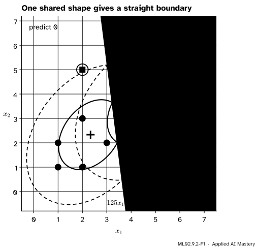
Give both classes the same ellipse and slide one copy over to the other mean. The two clouds are now identical apart from a shift. Walk along any straight line in the plane and the two densities rise and fall in the same way, one ahead of the other, so the place where they are equally high is a straight line too.
ML02.9.2-F1
Linear discriminant analysis on the twelve points. Both classes get the pooled covariance, so their ellipses are copies of each other and the boundary is the straight line \({125x_1 + 16x_2 = 462}\).
That straight line is linear discriminant analysis (LDA). It is one of the oldest classifiers in statistics, and it is still a strong, fast baseline: credit scoring and medical diagnosis used it for decades, and it remains the first thing to try when classes are few and examples are scarce.
Build it up
Step 1. Score each class in logs. As in the generative recipe of ML02.9.1, predict the class with the largest \({\pi_k\,N(\vect{x};\,\vect{\mu}_k, \mat{\Sigma})}\). The log is easier, and the largest stays the largest:
Step 2. Drop what every class shares. With one \(\mat{\Sigma}\) for all classes, \({-\ln(2\pi)}\) and \({-\tfrac12\ln\det\mat{\Sigma}}\) are the same in every score. They cannot change which score is largest.
Step 3. Open the bracket. The quadratic form contains a part with \(\vect{x}\) twice, a part with \(\vect{x}\) once and a part without it. The part with \(\vect{x}\) twice, \({\vect{x}\T\mat{\Sigma}^{-1}\vect{x}}\), does not depend on \(k\), so it drops out too. What is left is linear in \(\vect{x}\).
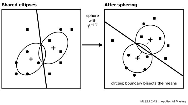
Step 4. See it as nearest mean. The picture behind the algebra: stretch the plane so that the shared ellipse becomes a circle. Then every class is a round cloud of the same size, and the closest mean wins (adjusted for the priors). The boundary between two round clouds of equal size is the perpendicular bisector of their means, a straight line, and stretching back keeps it straight.
ML02.9.2-F2
Sphering. After the plane is stretched so that the shared covariance becomes the identity, LDA is “pick the nearest mean”, and the boundary is the perpendicular bisector of the two means.
The formal statement
NoteDefinition: linear discriminant analysis
Model each class as \({N(\vect{\mu}_k, \mat{\Sigma})}\) with one covariance shared by all classes, and priors \(\pi_k\). The linear discriminant function of class \(k\) is
The two middle terms are equal. Each is a single number, a number is its own transpose, and \(\mat{A}\) is symmetric because \(\mat{\Sigma}\) is, so \({\vect{\mu}_k\T\mat{A}\vect{x} = (\vect{\mu}_k\T\mat{A}\vect{x})\T = \vect{x}\T\mat{A}\vect{\mu}_k}\). Hence
The first term is the same for every class and drops out. Adding \({\ln\pi_k}\) to the other two gives \({\delta_k(\vect{x})}\). It is linear in \(\vect{x}\): a weight vector \({\mat{\Sigma}^{-1}\vect{\mu}_k}\) and an intercept.
Two classes: the log-odds are linear. The log-odds of class 1 against class 0 are \({\delta_1(\vect{x}) - \delta_0(\vect{x})}\), because the shared parts cancelled in both. Subtract:
For a symmetric \(\mat{A}\) the bracket factorises as \({(\vect{\mu}_1 + \vect{\mu}_0)\T\mat{A}(\vect{\mu}_1 - \vect{\mu}_0)}\) (exercise 2). So the log-odds are \({\vect{w}\T\vect{x} + b}\) with
and the posterior is \({p(1 \mid \vect{x}) = \sigma(\vect{w}\T\vect{x} + b)}\), the sigmoid of ML01.6. LDA has exactly the form of logistic regression. The boundary \({\vect{w}\T\vect{x} + b = 0}\) is a straight line, a plane or a hyperplane, depending on the number of features.
Estimating the shared covariance. Each class contributes the scatter of its points about its own mean. The maximum-likelihood pooled covariance adds them up and divides by the number of points:
where \({\vect{v}_i = \vect{x}_i - \hat{\vect{\mu}}_k}\) is the deviation of a point from its own class mean.
It is the class covariances of ML02.9.1, averaged with weights \({n_k/n}\). The double sum \(\mat{S}_W\) is the within-class scatter matrix, which returns in ML02.9.4. Textbooks such as ESL divide by \({n - K}\) instead, which removes a small bias; scikit-learn divides by \(n\). With equal priors the boundary is the same either way. With unequal priors the cut moves a little, because rescaling \(\hat{\mat{\Sigma}}\) rescales \(\vect{w}\) but not \({\ln(\pi_1/\pi_0)}\).
Worked example
Fit LDA to the twelve points, with priors \({\pi_0 = \pi_1 = 1/2}\), and classify \({(3, 3)}\).
Scatter. Class 0’s scatter is six times its covariance, \({\tfrac13\begin{bmatrix}34 & 28\\ 28 & 34\end{bmatrix}}\); class 1’s is \({\tfrac13\begin{bmatrix}28 & -5\\ -5 & 40\end{bmatrix}}\). Their sum is
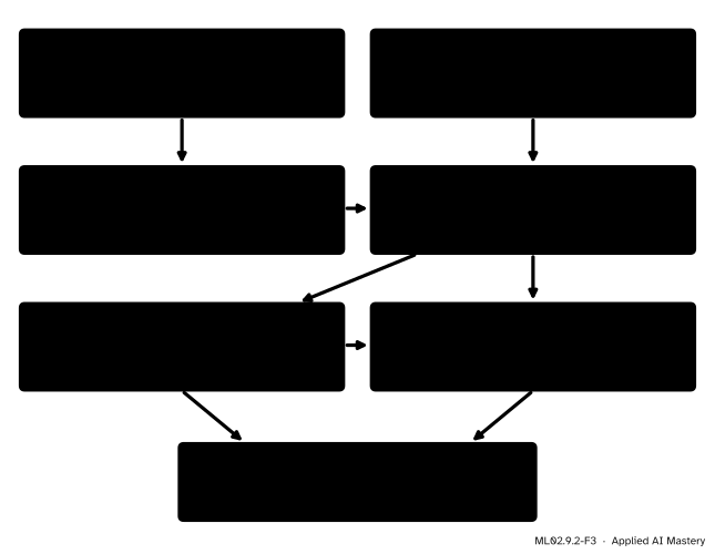
The worked example as a trace: from the scatter matrix to the weight vector, the intercept and the boundary.
Weight vector. The inverse of a 2 by 2 matrix swaps the diagonal, negates the off-diagonal and divides by the determinant. Here \({62 \cdot 74 - 23^2 = 4059}\), so
Boundary.\({\vect{w}\T\vect{x} + b = 0}\) means \({500x_1 + 64x_2 = 1848}\), or, dividing by 4, \({125x_1 + 16x_2 = 462}\). It passes through the midpoint of the means, \({(10/3, 17/6)}\), as it must with equal priors:
and the point goes to class 0. On the training set, 10 of 12 points are right; the two ringed in the anchor figure, \({(5, 5)}\) and \({(2, 5)}\), sit across the line.
Code
From scratch for any number of classes, then checked against scikit-learn.
import numpy as npfrom sklearn.discriminant_analysis import LinearDiscriminantAnalysisX = np.array([(1, 1), (2, 1), (1, 2), (2, 3), (3, 2), (5, 5), (4, 1), (5, 2), (5, 3), (4, 4), (2, 5), (6, 5)], dtype=float)y = np.array([0] *6+ [1] *6)def lda_fit(X, y): classes = np.unique(y) prior = np.array([np.mean(y == k) for k in classes]) means = np.array([X[y == k].mean(axis=0) for k in classes]) S_W =sum((X[y == k] - means[k]).T @ (X[y == k] - means[k]) for k in classes) Sigma = S_W /len(X) # pooled, maximum likelihood W = np.linalg.solve(Sigma, means.T) # column k is Sigma^-1 mu_k c =-0.5* np.sum(means.T * W, axis=0) + np.log(prior)return S_W, Sigma, W, cdef lda_scores(X, W, c):return X @ W + c # delta_k(x) for every row and classS_W, Sigma, W, c = lda_fit(X, y)w, b = W[:, 1] - W[:, 0], c[1] - c[0] # two classes: log-odds w.x + bprint("S_W x 3:", (3* S_W).round(4).tolist())print("w =", w.round(4), " w x 451 =", (451* w).round(4), " b =", round(b, 4))p33 =1/ (1+ np.exp(-(np.array([3.0, 3.0]) @ w + b)))right = (lda_scores(X, W, c).argmax(axis=1) == y).sum()print(f"P(class 1 | (3, 3)) = {p33:.4f}; training points right: {right} of 12")lda = LinearDiscriminantAnalysis().fit(X, y)print("scikit-learn coef_", lda.coef_.round(4), "intercept_", lda.intercept_.round(4),"P(1 | (3, 3))", lda.predict_proba([[3.0, 3.0]])[0, 1].round(4))
S_W x 3: [[62.0, 23.0], [23.0, 74.0]]
w = [1.1086 0.1419]  w x 451 = [500.  64.]  b = -4.0976
P(class 1 | (3, 3)) = 0.4144; training points right: 10 of 12
scikit-learn coef_ [[1.1086 0.1419]] intercept_ [-4.0976] P(1 | (3, 3)) 0.4144
For two classes, scikit-learn’s coef_ and intercept_ are the \(\vect{w}\) and \(b\) of the log-odds, and they match ours to every printed digit.
Now the same form fitted the other way. Logistic regression (ML01.6) also predicts \({\sigma(\vect{w}\T\vect{x} + b)}\), but it chooses \(\vect{w}\) and \(b\) to fit the labels directly. A very large C switches its penalty off almost entirely.
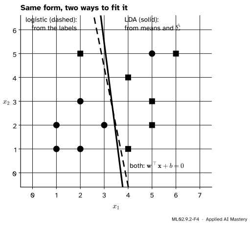
from sklearn.linear_model import LogisticRegressionlogreg = LogisticRegression(C=1e4, max_iter=10000).fit(X, y)w_lr, b_lr = logreg.coef_[0], logreg.intercept_[0]print("logistic regression: w =", w_lr.round(2), " b =", round(b_lr, 2)," right:", int(logreg.score(X, y) *12), "of 12")for name, (ww, bb) in (("LDA", (w, b)), ("logistic", (w_lr, b_lr))):print(f"{name:9s} boundary crosses x2 = 0 at x1 = {-bb / ww[0]:.2f} and x2 = 6 at x1 = {-(bb +6* ww[1]) / ww[0]:.2f}")
logistic regression: w = [0.9  0.18]  b = -3.51  right: 10 of 12
LDA       boundary crosses x2 = 0 at x1 = 3.70 and x2 = 6 at x1 = 2.93
logistic  boundary crosses x2 = 0 at x1 = 3.89 and x2 = 6 at x1 = 2.68
ML02.9.2-F4
Two straight boundaries of the same form. LDA computes its line from the means and the pooled covariance; logistic regression searches for the line that best fits the labels.
The two lines are close but not equal. When is each better? ESL (section 4.4.5) puts the difference this way: LDA fits the full joint likelihood of features and labels, so it also uses how the features are spread; logistic regression fits only \({p(y \mid \vect{x})}\). When the classes really are Gaussian with a shared covariance, LDA’s extra assumption buys efficiency (Efron’s estimate, quoted there: in the worst case, ignoring it costs about 30% more data for the same error), and ISLR (section 4.4) adds that LDA then tends to win with small samples and stays stable when the classes are well separated, where the logistic estimates become unstable. The price is robustness: points far from the boundary still pull on \(\hat{\mat{\Sigma}}\), so LDA is hurt by gross outliers, and logistic regression is the safer bet when the Gaussian picture is doubtful. In practice the two often agree closely, as here.
Explore
The ellipse explorer is in lesson ML02.9.3. Switch on Shared covariance: the boundary becomes a straight line. Then turn one class’s ellipse and watch the line turn as well, although neither mean has moved: the shared covariance, not only the means, sets the direction of the boundary.
Pitfalls
ML02.9.2-F5
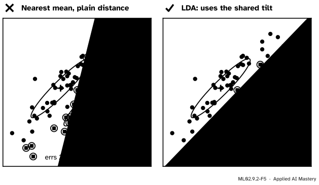
Wrong beside right, on two tilted clouds with a shared covariance. Ignoring the covariance cuts straight across both clouds; LDA cuts between them. The error rates are for the whole population.
“The LDA boundary is the perpendicular bisector of the two means.”
Not in general. The boundary is at right angles to \({\vect{w} = \mat{\Sigma}^{-1}(\vect{\mu}_1 - \vect{\mu}_0)}\), not to \({\vect{\mu}_1 - \vect{\mu}_0}\). The two directions agree when the shared covariance is a multiple of the identity (and then, with equal priors, the boundary is the bisector; ESL makes this remark in its discussion of Figure 4.5), or more generally when \({\vect{\mu}_1 - \vect{\mu}_0}\) happens to be an eigenvector of \(\mat{\Sigma}\). For long tilted clouds the difference is large: the nearest-mean rule errs 22% of the time, LDA 2%.
“LDA and logistic regression have the same form, so they give the same model.”
Same form, different fit. LDA plugs estimated means and a pooled covariance into a formula; logistic regression maximises the likelihood of the labels. They differ most when the data are not Gaussian or have outliers, and on data that a line separates perfectly, where the logistic estimates do not exist but LDA’s do.
“With unequal class sizes the boundary still passes through the midpoint of the means.”
The prior term \({\ln(\pi_1/\pi_0)}\) shifts it. A rarer class needs stronger evidence, so the line moves towards the rarer class’s mean (exercise 1), just as the threshold did in ML02.6.1.
Check yourself
Recall
1. Which assumption makes the discriminant functions linear?
Show answer
All classes share one covariance matrix \(\mat{\Sigma}\). Then \({\vect{x}\T\mat{\Sigma}^{-1}\vect{x}}\) and \({\ln\det\mat{\Sigma}}\) are the same for every class and drop out.
2. Write the linear discriminant function \(\delta_k(\vect{x})\).
Add up each class’s scatter about its own mean, and divide by \(n\) (maximum likelihood, as scikit-learn does) or by \({n - K}\) (the unbiased version in ESL). Equivalently, average the class covariances with weights \({n_k/n}\).
4. For two classes, what are \(\vect{w}\) and \(b\) in the log-odds \({\vect{w}\T\vect{x} + b}\)?
5. Name one situation that favours LDA and one that favours logistic regression.
Show answer
LDA: few examples and roughly Gaussian classes, or well-separated classes. Logistic regression: data far from Gaussian or with gross outliers.
Exercises
1.★ For the twelve points, keep the means and \(\hat{\mat{\Sigma}}\) but set \({\pi_1 = 1/4}\). Find the new boundary and classify \({(4, 2)}\) under both priors.
Show solution
Only \(b\) changes, by \({\ln(\pi_1/\pi_0) = \ln(1/3) = -1.099}\). Since \({\vect{w}\T\vect{x} = 4(125x_1 + 16x_2)/451}\), the boundary \({\vect{w}\T\vect{x} = 1848/451 + \ln 3}\) becomes
At \({(4, 2)}\), \({125 \cdot 4 + 16 \cdot 2 = 532}\). That is above 462, so with equal priors the point goes to class 1; it is below 585.9, so with \({\pi_1 = 1/4}\) it goes to class 0. The line has moved right, towards the rarer class.
2.★★ Show that for a symmetric matrix \(\mat{A}\),
The two middle terms are numbers, and transposing one gives the other because \({\mat{A}\T = \mat{A}}\): \({\vect{\mu}_0\T\mat{A}\vect{\mu}_1 = \vect{\mu}_1\T\mat{A}\T\vect{\mu}_0 = \vect{\mu}_1\T\mat{A}\vect{\mu}_0}\). So they cancel and the left-hand side remains. It is the matrix version of \({a^2 - c^2 = (a + c)(a - c)}\).
3.★★★ Suppose \({\mat{\Sigma} = s^2\mat{I}}\) and the priors are equal. Show that LDA assigns \(\vect{x}\) to the class with the nearest mean, and that the two-class boundary is the perpendicular bisector of the means.
Show solution
With \({\mat{\Sigma}^{-1} = \mat{I}/s^2}\) and equal \({\ln\pi_k}\), which drop out,
The first term is the same for every class, so the largest \(\delta_k\) belongs to the smallest distance \({\norm{\vect{x} - \vect{\mu}_k}}\). The boundary between two classes is the set of points equally far from both means, which is the perpendicular bisector of the segment joining them.
Summary card
One shared covariance: the quadratic terms cancel and the boundary is a straight line.
Pooled covariance:\({\hat{\mat{\Sigma}} = \sum_k (n_k/n)\hat{\mat{\Sigma}}_k}\).
Two classes:\({p(1 \mid \vect{x}) = \sigma(\vect{w}\T\vect{x} + b)}\) with \({\vect{w} = \mat{\Sigma}^{-1}(\vect{\mu}_1 - \vect{\mu}_0)}\).
Versus logistic regression: same form, fitted from the joint likelihood instead of the labels alone.
Sources and next steps
Sources. Each was opened and checked against this lesson on 15 November 2026.
T. Hastie, R. Tibshirani and J. Friedman, The Elements of Statistical Learning, 2nd edition, corrected 12th printing (2017). Section 4.3: the linear discriminant functions, equation (4.10); the estimates of \(\pi_k\), \(\mu_k\) and the pooled covariance divided by \({N - K}\); the remark under Figure 4.5 that the boundaries are perpendicular bisectors only for a spherical covariance and equal priors; section 4.3.2 on sphering. Section 4.4.5: LDA and logistic regression have the same linear log-odds (4.33, 4.34) but are fitted by the full and the conditional likelihood; Efron’s 30% efficiency result; LDA is not robust to gross outliers; with separable data the logistic estimates are undefined.
G. James, D. Witten, T. Hastie and R. Tibshirani, An Introduction to Statistical Learning, 2nd edition (with R). Section 4.4: three reasons to prefer LDA (instability of logistic regression under substantial separation, small samples with roughly normal predictors, more than two classes); section 4.4.2: the discriminant function (4.24).
scikit-learn, Linear and Quadratic Discriminant Analysis, User Guide section 1.2 (the LDA log posterior and its coef_ and intercept_), and the LinearDiscriminantAnalysis reference: covariance_ is the weighted within-class covariance \({\sum_k \text{prior}_k C_k}\) built from the biased class covariances.