Swap the dot product in the SVM’s dual for a kernel and the boundary bends. Solve the quadratic-kernel SVM on the rings by hand, build a kernel SVM from scratch and match scikit-learn’s SVC, and learn how gamma and C shape an RBF boundary.
ML02.8.3L2 Intermediate30 minIn review (what this means)
The maths and code on this page are checked by automated tests on every change, but an independent reader has not signed it off yet. Spot a mistake or a confusing step? Tell us.
Kernelise the soft-margin dual and write the decision function as a sum over the support vectors.
Solve the quadratic-kernel SVM on the rings by hand and recover the circle of radius 2.12.
Build a kernel SVM from scratch with SLSQP and match scikit-learn’s SVC.
Explain how gamma and C shape an RBF boundary, and choose them by cross-validated grid search.
The question
The SVM of ML02.7 draws the widest straight street between two classes. On the rings that is useless: no straight street exists. The last lesson found that the SVM’s dual only ever asks for dot products. What happens if we answer it with a kernel instead, and how do we control the curves it then draws?
From the last lesson
1. Which feature map does the kernel \({(\vect{x} \cdot \vect{z})^2}\) belong to in the plane?
2. What does a larger \(\gamma\) do to the RBF kernel \({e^{-\gamma \norm{\vect{x} - \vect{z}}^2}}\)?
Show answer
It makes the kernel fall faster with distance, a shorter length scale \({\ell = 1/\sqrt{2\gamma}}\): only close neighbours count as similar.
Intuition
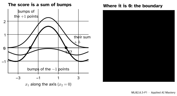
ML02.7.2 found that a trained SVM scores a new point \(\vect{x}\) by \({\sum_i \alpha_i y_i\, \vect{x}_i \cdot \vect{x} + b}\), a weighted sum over the support vectors. Replace each dot product by a kernel and the score becomes a sum of kernel values. With the RBF kernel, each support vector contributes a bump centred on itself: pushing the score up if it is a \(+1\) point, down if it is a \(-1\) point, by an amount set by its weight \(\alpha_i\).
ML02.8.3-F1
Left: along the \(x_1\) axis, the bumps of the inner points push the score up and those of the outer points push it down; with the bias added, the sum crosses zero near \({\pm 1.77}\). Right: the zero line of the score over the whole plane is the boundary.
Nothing in this picture needed the lifted points. The SVM is trained and used with kernel values alone, so the lift can have three coordinates or infinitely many: the cost is the same.
Build it up
Step 1. The dual, as ML02.7.3 left it. For training points \({\vect{x}_i}\) with labels \({y_i \in \{-1, +1\}}\) and a penalty \(C\), the soft-margin SVM finds weights \({\alpha_i}\) that maximise
subject to \({0 \le \alpha_i \le C}\) and \({\sum_i \alpha_i y_i = 0}\).
Step 2. Train on lifted points. Run the same SVM on \({\varphi(\vect{x}_i)}\) instead of \({\vect{x}_i}\). Every \({\vect{x}_i \cdot \vect{x}_j}\) becomes \({\varphi(\vect{x}_i) \cdot \varphi(\vect{x}_j) = k(\vect{x}_i, \vect{x}_j)}\): the entries of the Gram matrix. The solver never sees anything else.
Step 3. Score without the weight vector. The weight vector now lives in the lifted space, \({\vect{w} = \sum_i \alpha_i y_i \varphi(\vect{x}_i)}\), and for the RBF kernel it has infinitely many coordinates. But the score only needs its dot product with \({\varphi(\vect{x})}\), and that splits into kernel values: \({\vect{w} \cdot \varphi(\vect{x}) = \sum_i \alpha_i y_i\, k(\vect{x}_i, \vect{x})}\).
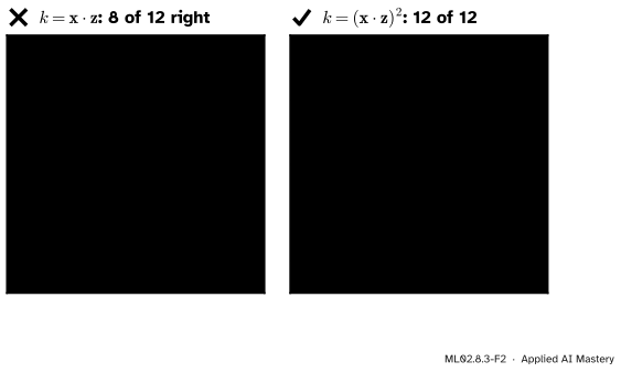
Step 4. Same solver, different kernel. Hand the solver the plain dot product and the rings defeat it. Hand it the square of the dot product and it draws a circle.
ML02.8.3-F2
The same solver on the rings. Left: with the plain dot product the best it can do is \({\vect{w} = \vect{0}}\), calling every point \(-1\). Right: with \({(\vect{x} \cdot \vect{z})^2}\) it finds the circle of the first lesson.
The formal statement
NoteThe kernel SVM
Given a kernel \(k\) and a penalty \(C\), find \({\alpha_1, \dots, \alpha_n}\) that maximise
The problem is the dual of ML02.7.3 with the Gram matrix in place of the dot products, so all of its facts carry over. Points with \({\alpha_i = 0}\) drop out of the sum; the others are the support vectors. A point with \({0 < \alpha_i < C}\) sits exactly on the margin, which is what fixes \(b\).
The bias. For such a point \({\vect{x}_s}\), the margin condition is \({y_s f(\vect{x}_s) = 1}\). Multiply both sides by \(y_s\) and use \({y_s^2 = 1}\):
In practice \(b\) is averaged over all such points, to smooth out rounding.
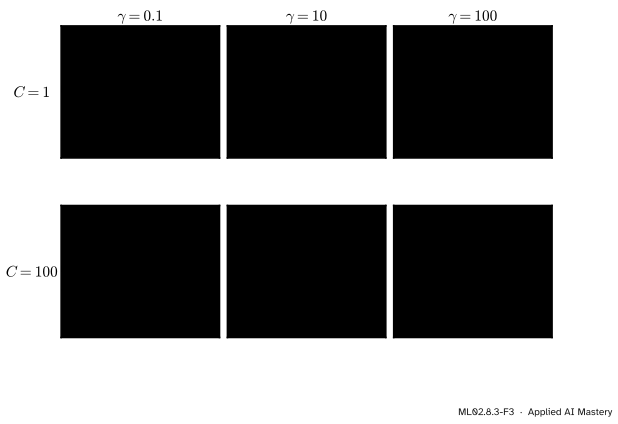
How \(\gamma\) and \(C\) shape an RBF boundary. Each support vector adds a bump of width about \({\ell = 1/\sqrt{2\gamma}}\). A small \(\gamma\) gives wide bumps that blend into a smooth, gently curving boundary. A large \(\gamma\) gives narrow bumps, and the boundary wraps each training point in its own island. \(C\) is the price of a point inside the margin or on the wrong side (ML02.7.3): a small \(C\) tolerates mistakes and keeps the boundary simple, a large \(C\) bends it to classify the training points.
ML02.8.3-F3
One RBF SVM on 60 moons points, with six settings. Each panel gives its accuracy on 400 fresh points. Too small a \(\gamma\) underfits; too large a \(\gamma\) wraps the training points.
Neither number can be read off the data, so both are chosen by cross-validation (ML01.9.3). Because each acts by orders of magnitude, the grid of candidates is spaced by factors of 10, and scikit-learn’s GridSearchCV tries every pair.
Worked example
The quadratic-kernel SVM on the rings, with a hard margin, solved by hand.
The kernel \({(\vect{x} \cdot \vect{z})^2}\) belongs to the map \({\varphi(\vect{x}) = (x_1^2, \sqrt{2}\,x_1 x_2, x_2^2)}\), so we can solve the problem in that three-dimensional space and check it against the kernel form.
Symmetry. Swapping \(x_1\) and \(x_2\) leaves the rings unchanged, and so does flipping the sign of \(x_1\). The widest street is unique (ML02.7.1: the objective \({\frac{1}{2}\norm{\vect{w}}^2}\) has one lowest point), so it must be unchanged too. In lifted coordinates the swap exchanges \(z_1\) and \(z_3\), which forces \({w_1 = w_3}\); the flip changes the sign of \(z_2\), which forces \({w_2 = 0}\). So \({\vect{w} = (a, 0, a)}\) and the score is \({a\,(x_1^2 + x_2^2) + b}\).
Constraints. Each point must score at least 1 on its own side. The inner points have \({x_1^2 + x_2^2 = 1}\), the diagonal points 8 and the axis points 9:
\[
\begin{aligned}
a + b &\ge 1, \\
-(8a + b) &\ge 1, \\
-(9a + b) &\ge 1 .
\end{aligned}
\]
Widest street. Minimise \({\frac{1}{2}\norm{\vect{w}}^2 = a^2}\). The first two lines need \(a < 0\), so write \({a = -A}\) with \({A > 0}\). They become \({b \ge 1 + A}\) and \({b \le 8A - 1}\), which can both hold only when \({1 + A \le 8A - 1}\), that is \({A \ge 2/7}\). The smallest is \({A = 2/7}\), and then both bounds give \({b = 9/7}\). The third line holds with room to spare: \({18/7 - 9/7 = 9/7 \ge 1}\).
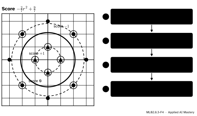
The score is \({-\frac{2}{7}(x_1^2 + x_2^2) + \frac{9}{7}}\). It is zero on the circle \({x_1^2 + x_2^2 = 4.5}\), exactly the cut of the first lesson, now found as the widest street.
Dual weights. The axis points are off the margin, so their \({\alpha_i = 0}\). By symmetry give each inner point weight \(p\) and each diagonal point weight \(q\). The constraint \({\sum_i \alpha_i y_i = 4p - 4q = 0}\) gives \({p = q}\). The four inner points lift to \({(1, 0, 0)}\) twice and \({(0, 0, 1)}\) twice, which add to \({(2, 0, 2)}\); the four diagonal points lift to \({(4, \pm 4\sqrt{2}, 4)}\), which add to \({(16, 0, 16)}\). So
and \({-14p = -2/7}\) gives \({p = 1/49}\) on each of the eight support vectors.
ML02.8.3-F4
The hand solution. The street’s two edges are the circles through the inner points (score \(+1\)) and the diagonal points (score \(-1\)); the boundary halfway between, in score, is the circle of radius 2.12.
Check in kernel form. At the new point \({(0.5, 0.5)}\), the kernel values with the inner points are \({0.5^2 = 0.25}\) each, and with the diagonal points \({2^2 = 4}\), \(0\), \(0\) and \({(-2)^2 = 4}\). So
The two solvers agree on the boundary, \(b\) and the total weight \({\sum \alpha_i = 8/49}\), but not on the weights themselves. SVC puts \({2/49}\) on four points, one from each mirror pair. That is allowed: \({\varphi(1, 0) = \varphi(-1, 0)}\) and \({\varphi(2, 2) = \varphi(-2, -2)}\), so a weight can be moved between twins without changing \(\vect{w}\).
Now the RBF kernel on 60 points of make_moons, with 400 fresh points as a test set.
from sklearn.datasets import make_moonsfrom sklearn.model_selection import GridSearchCV, StratifiedKFoldX, y01 = make_moons(60, noise=0.2, random_state=3)Xt, yt01 = make_moons(400, noise=0.2, random_state=103)y, yt =2.0* y01 -1, 2.0* yt01 -1# labels -1 and +1a, b = fit_kernel_svm(rbf(X, X, 1.0), y, C=1.0)f_scratch = (a * y) @ rbf(X, Xt, 1.0) + bsvc = SVC(kernel="rbf", gamma=1.0, C=1.0).fit(X, y)print("support vectors: from scratch", np.sum(a >1e-6), " SVC", len(svc.support_))print("largest gap between the two scores:", f"{np.abs(f_scratch - svc.decision_function(Xt)).max():.1e}")print("test accuracy:", np.mean(np.sign(f_scratch) == yt), svc.score(Xt, yt))for C in [1, 100]: row = [SVC(gamma=g, C=C).fit(X, y) for g in [0.1, 10, 100]]print(f"C = {C:3d} train", [round(m.score(X, y), 3) for m in row], " test", [round(m.score(Xt, yt), 3) for m in row])search = GridSearchCV(SVC(), {"C": [0.1, 1, 10, 100], "gamma": [0.1, 1, 10, 100]}, cv=StratifiedKFold(5, shuffle=True, random_state=0)).fit(X, y)print("best:", search.best_params_, " CV accuracy", round(search.best_score_, 3)," test accuracy", search.score(Xt, yt))from sklearn.pipeline import make_pipelinefrom sklearn.preprocessing import StandardScalerunit = np.array([100.0, 1.0]) # the first feature in a 100 times larger unitraw = SVC(gamma=10, C=1).fit(X * unit, y)scaled = make_pipeline(StandardScaler(), SVC(gamma=10, C=1)).fit(X * unit, y)print("first feature times 100: raw train", raw.score(X * unit, y), " raw test", raw.score(Xt * unit, yt)," standardised test", scaled.score(Xt * unit, yt))
support vectors: from scratch 26  SVC 26
largest gap between the two scores: 4.7e-04
test accuracy: 0.905 0.905
C =   1  train [0.85, 0.983, 1.0]  test [0.835, 0.96, 0.858]
C = 100  train [0.917, 1.0, 1.0]  test [0.882, 0.958, 0.86]
best: {'C': 1, 'gamma': 10}  CV accuracy 0.983  test accuracy 0.96
first feature times 100: raw train 1.0  raw test 0.555  standardised test 0.95
The scratch solver and SVC pick the same 26 support vectors, and their scores agree to within about 0.001: SVC’s solver stops at a tolerance of \({10^{-3}}\) by default. The table shows the figure’s story in numbers. With \({C = 1}\), \({\gamma = 0.1}\) is right on only 85% of its own training points; \({\gamma = 100}\) gets all of them and only about 86% of the test points; \({\gamma = 10}\) sits between, near 96% on the test set. Five-fold cross-validation on the 60 training points picks \({C = 1}\) and \({\gamma = 10}\) without seeing the test set.
Explore
ML02.8-X1
Kernel lift
Start in lift mode: turn the view and slide the plane height. Every height between 1 and 8 splits the lifted rings, and the circle it draws in the plane has radius \({\sqrt{h}}\). Then switch to RBF SVM and slide gamma from left to right.
In lift mode, watch the read-out as the plane passes heights 1 and 8: at 1 or below, or at 8 or above, some points are no longer on their own side. In RBF mode, the right-hand view shows the score as a surface over the plane, and the boundary is where the flat plane at height 0 cuts it. Small \(\gamma\) gives one smooth loop round the four inner points. Near \({\gamma = 2.8}\) the score at the centre of the ring drops below zero and a hole opens in the middle of the loop. Near \({\gamma = 4.2}\) the gaps between neighbouring inner points drop below zero too, and the ring breaks into islands, one round each inner point.
Pitfalls
ML02.8.3-F5
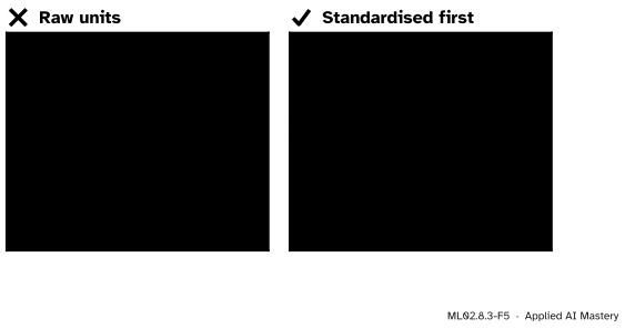
Wrong beside right. The first feature is multiplied by 100, as if measured in centimetres instead of metres. Left: on the raw numbers, distance is all first feature and the kernel ignores the second. Right: standardised first, the same SVM recovers the moons.
“A kernel SVM does not care about the units of the features.”
The RBF kernel is built from distances, and a feature measured in large numbers dominates every distance, exactly as in k-nearest neighbours (ML01.3.3). With the first moons feature multiplied by 100, an RBF SVM with \({\gamma = 10}\) still fits all 60 training points but is right on only about 56% of the test points. Put a StandardScaler in front of the SVM in a pipeline, and it is right on 95% again.
“The setting with the best training accuracy is the best setting.”
A large enough \(\gamma\) wraps every training point in its own island and reaches 100% training accuracy for any labels at all. On the moons, \({\gamma = 100}\) does exactly that and loses ten points of test accuracy. Choose \(\gamma\) and \(C\) by cross-validation, never by training accuracy.
“The weights \(\alpha_i\) are unique, so they tell you which points matter.”
The boundary and the score are unique; the weights need not be. On the rings, SLSQP spreads \({1/49}\) over eight points and SVC puts \({2/49}\) on four, because twin points have the same lifted image. Read the support vectors as one valid explanation of the boundary, not the only one.
Check yourself
Recall
1. What changes in the SVM’s dual when a kernel is used?
Show answer
Every dot product \({\vect{x}_i \cdot \vect{x}_j}\) is replaced by \({k(\vect{x}_i, \vect{x}_j)}\). The constraints \({0 \le \alpha_i \le C}\) and \({\sum_i \alpha_i y_i = 0}\) stay as they were.
2. How does a kernel SVM score a new point, and why does it never need \({\varphi}\)?
Show answer
\({f(\vect{x}) = \sum_i \alpha_i y_i\, k(\vect{x}_i, \vect{x}) + b}\). The weight vector \({\sum_i \alpha_i y_i \varphi(\vect{x}_i)}\) only ever appears in a dot product with \({\varphi(\vect{x})}\), and each such product is a kernel value.
3. How is \(b\) found?
Show answer
From a support vector strictly inside the box, \({0 < \alpha_s < C}\), which lies on the margin: \({b = y_s - \sum_i \alpha_i y_i\, k(\vect{x}_i, \vect{x}_s)}\), averaged over all such points.
4. What does the quadratic-kernel SVM find on the rings?
Show answer
The score \({-\frac{2}{7}(x_1^2 + x_2^2) + \frac{9}{7}}\): the circle of radius 2.12, with the four inner and four diagonal points as support vectors.
5. What do a very small and a very large \(\gamma\) do to an RBF boundary?
Show answer
A very small \(\gamma\) gives wide bumps and a smooth, nearly straight boundary that can underfit. A very large \(\gamma\) gives narrow bumps and islands round single training points that overfit.
Exercises
1.★ Use the hand solution of the worked example to classify the point \((2, 1)\), once with the formula \({-\frac{2}{7}r^2 + \frac{9}{7}}\) and once with the kernel sum.
Show solution
Formula: \({r^2 = 5}\), so \({f = -\frac{10}{7} + \frac{9}{7} = -\frac{1}{7}}\), class \(-1\).
Kernel sum: the dot products of \((2, 1)\) with the inner points are 2, \(-2\), 1 and \(-1\), whose squares add to \({4 + 4 + 1 + 1 = 10}\). With the diagonal points they are 6, 2, \(-2\) and \(-6\), whose squares add to \({36 + 4 + 4 + 36 = 80}\). So \(f = \frac{10}{49} - \frac{80}{49} + \frac{9}{7} = -\frac{70}{49} + \frac{63}{49} = -\frac{1}{7}\), the same.
2.★★ The RBF length scale is \({\ell = 1/\sqrt{2\gamma}}\). Find \(\ell\) for \({\gamma = 0.5}\) and for \({\gamma = 10}\), and the kernel value between the inner ring points \((1, 0)\) and \((0, 1)\), which are \({\sqrt{2}}\) apart. Why does the boundary break into islands for \({\gamma = 10}\)?
Show solution
For \({\gamma = 0.5}\), \({\ell = 1/\sqrt{1} = 1}\); for \({\gamma = 10}\), \({\ell = 1/\sqrt{20} \approx 0.22}\). At distance \({\sqrt{2}}\), the kernel is \({e^{-0.5 \times 2} = e^{-1} \approx 0.37}\) for \({\gamma = 0.5}\) but \({e^{-10 \times 2} = e^{-20} \approx 2 \times 10^{-9}}\) for \({\gamma = 10}\). With \({\gamma = 10}\) the bumps of the inner points barely reach each other, so between them, at the centre, the score falls back to \(b\), which is negative. Each inner point keeps a small island of its own.
3.★★★ For a hard-margin kernel SVM, show that \({\sum_i \alpha_i = \norm{\vect{w}}^2}\), where \({\vect{w} = \sum_i \alpha_i y_i \varphi(\vect{x}_i)}\). Check it on the rings and find the width of the street in the lifted space.
Show solution
Complementary slackness (ML02.7.2) says \({\alpha_i\,[\,y_i(\vect{w} \cdot \varphi(\vect{x}_i) + b) - 1\,] = 0}\) for every \(i\). Add these up over \(i\) and move the \(-\alpha_i\) terms across:
On the rings, \({\sum_i \alpha_i = 8/49}\) and \({\norm{\vect{w}}^2 = 2 \times (2/7)^2 = 8/49}\). The street is \({2/\norm{\vect{w}} = 2 \times 7 / \sqrt{8} = 7/\sqrt{2} \approx 4.95}\) wide in the lifted space.
Summary card
A kernel SVM is the SVM’s dual with the Gram matrix in place of the dot products.
Settings.\(\gamma\) sets the bump width, \(C\) the price of mistakes; choose both by cross-validation on a log grid, after scaling.
Sources and next steps
Sources. Each was opened and checked against this lesson on 15 November 2026.
Tengyu Ma and Andrew Ng, CS229 Lecture Notes, Stanford University, Section 6.6. Writes the SVM’s prediction as \({\sum_i \alpha_i y^{(i)} \langle x^{(i)}, x\rangle + b}\) (equation 6.15), notes that only the support vectors have non-zero \(\alpha_i\), and that the whole algorithm can be written in inner products, which is what lets kernels in.
Gareth James, Daniela Witten, Trevor Hastie, Robert Tibshirani and Jonathan Taylor, An Introduction to Statistical Learning with Applications in Python, Section 9.3.2. Replaces the inner product by a kernel (9.20), gives the polynomial (9.22) and radial (9.24) kernels and the SVM’s function as a sum over the support vectors (9.23), and explains that the radial kernel is local: far-away training points play essentially no part in a prediction.
scikit-learn 1.9 User Guide, Section 1.4, Support Vector Machines. Section 1.4.7.1 gives SVC’s dual with \({Q_{ij} = y_i y_j K(x_i, x_j)}\), the box \({0 \le \alpha_i \le C}\) and the decision function as a sum over the support vectors plus \(b\). Section 1.4.6.1 says that a low C makes the decision surface smooth, that a larger gamma means other examples must be closer to be affected, and advises GridSearchCV with C and gamma spaced exponentially. Section 1.4.5 says SVMs are not scale invariant and recommends scaling in a Pipeline.
Kilian Weinberger, Lecture 14: Kernels continued, Cornell CS4780 (Fall 2018). Gives the kernel SVM’s dual with the box constraint and the classifier \({\operatorname{sign}\big(\sum_i \alpha_i y_i k(x_i, x) + b\big)}\).