Four points inside a ring of eight cannot be split by any line. Add one coordinate, the squared distance from the origin, and a flat plane splits them. See why, what that plane is back in the plane, and what lifting by hand costs.
ML02.8.1L2 Intermediate25 minIn review (what this means)
The maths and code on this page are checked by automated tests on every change, but an independent reader has not signed it off yet. Spot a mistake or a confusing step? Tell us.
Prove that no line separates the rings, and show that the lift z = x1^2 + x2^2 makes them separable by a plane.
Translate a plane in the lifted space back into a curve in the original plane by completing the square.
Compute the quadratic map (x1^2, sqrt(2) x1 x2, x2^2) by hand and classify points with a linear rule on it.
Count the coordinates of a polynomial lift with a binomial coefficient and explain why the count limits lifting by hand.
Fit a linear classifier on lifted features in NumPy and scikit-learn and check that it separates the rings.
The question
Four points sit inside a ring of eight. Any child can draw a circle round the four. Yet logistic regression, given these twelve points, gives up: it calls every point an outsider and is right only 8 times in 12. A linear model can only draw straight lines. Is there a way to let it draw the circle without changing the model at all?
Intuition
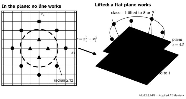
The points are the course’s rings. Class \(+1\) sits at \((1, 0)\), \((-1, 0)\), \((0, 1)\) and \((0, -1)\). Class \(-1\) sits at \((\pm 3, 0)\), \((0, \pm 3)\) and \((\pm 2, \pm 2)\). Inside and outside differ in one thing: how far a point is from the origin.
So give each point a third coordinate, its squared distance from the origin, \({z = x_1^2 + x_2^2}\), and stand it at that height. The inner points rise to height 1. The outer ones rise to 8 or 9.
ML02.8.1-F1
Left: no straight line puts the four triangles on one side and the eight circles on the other. Right: lift every point to the height \({x_1^2 + x_2^2}\) and the flat plane \(z = 4.5\) does it. Seen from above, that plane cuts the bowl in the dashed circle on the left.
In the lifted space the job is easy. Any flat plane at a height between 1 and 8 has the inner points below it and the outer points above it. A flat plane is exactly what a linear model draws in three dimensions. And when you look back down at the plane, the place where the flat plane cuts the bowl is a circle.
That is the whole idea of this module. Do not bend the model. Lift the data until a straight cut works. The model stays linear in the lifted coordinates, while its boundary, seen in the original ones, curves.
Build it up
Step 1. No line works. Suppose some line \({w_1 x_1 + w_2 x_2 + b = 0}\) had the inner points on its positive side and the outer points on its negative side. Then for \((1, 0)\) and \((-1, 0)\)
\[
\begin{aligned}
w_1 + b &> 0, \\
-w_1 + b &> 0 .
\end{aligned}
\]
Adding them gives \(2b > 0\). For \((3, 0)\) and \((-3, 0)\) we need
\[
\begin{aligned}
3w_1 + b &< 0, \\
-3w_1 + b &< 0 ,
\end{aligned}
\]
and adding gives \(2b < 0\). Both cannot hold, so no such line exists. The trouble is symmetry: each class surrounds the same centre, so a line that favours one side of the centre for one class favours it for the other too.
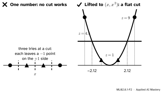
Step 2. The same puzzle, one dimension down. Put four points on a number line: \(+1\) at \(x = \pm 1\) and \(-1\) at \(x = \pm 3\). No single cut works. Now lift each \(x\) to the point \({(x, x^2)}\) on a parabola.
ML02.8.1-F2
Left: on the line, every cut leaves a \(-1\) point with the \(+1\) points. Right: on the parabola the inner points are low and the outer ones high, and the horizontal line \(z = 4.5\) splits them. It meets the parabola above \(x = \pm 2.12\).
Step 3. Back to the plane. Do the same with two features. The new coordinate \({z = x_1^2 + x_2^2}\) is the squared distance from the origin. A point lifted to height \(z\) lies on the bowl \({z = x_1^2 + x_2^2}\), the parabola spun round its axis.
Step 4. A flat cut. In the lifted space the rule “predict \(+1\) when \(z < 4.5\)” is linear: it uses the weights \((0, 0, -1)\) on the three coordinates \((x_1, x_2, z)\) and the bias \(4.5\). The inner points score \({4.5 - 1 = 3.5}\). The outer ones score \(4.5 - 8 = -3.5\) or \(4.5 - 9 = -4.5\).
Step 5. Look back down. The points where the score is zero satisfy \({x_1^2 + x_2^2 = 4.5}\): a circle of radius \({\sqrt{4.5} \approx 2.12}\). The rule is linear in the lifted coordinates and circular in the original ones.
The formal statement
NoteDefinition: feature map
A feature map is a function \({\varphi : \R^d \to \R^D}\) that turns each input \(\vect{x}\) into a longer list of features \({\varphi(\vect{x})}\). A linear model on lifted features scores an input by
\[
s(\vect{x}) = \vect{w} \cdot \varphi(\vect{x}) + b ,
\]
with \({\vect{w}}\) in \(\R^D\), and predicts \(+1\) when \({s(\vect{x}) > 0}\).
Logistic regression, the perceptron and the SVM all work unchanged on \({\varphi(\vect{x})}\): they see a table with \(D\) columns instead of \(d\). Training is the same convex problem as before, because the score is still linear in the weights.
NoteResult: a plane in the lift is a circle in the plane
Take \({\varphi(\vect{x}) = (x_1,\; x_2,\; x_1^2 + x_2^2)}\). If \(w_3 \ne 0\), the boundary \({s(\vect{x}) = 0}\) is a circle (or a single point, or nothing), centred at \({(-w_1 / 2w_3,\; -w_2 / 2w_3)}\). If \(w_3 = 0\), it is a line.
The left side is the squared distance from the point \({(-w_1/2w_3,\; -w_2/2w_3)}\). When the right side is positive, the boundary is the circle of that radius squared round that centre; when it is zero, a single point; when it is negative, no point at all. If \(w_3 = 0\) the squares vanish from the start and the boundary is the line \({w_1 x_1 + w_2 x_2 + b = 0}\).
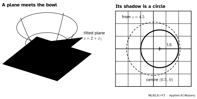
A tilted plane gives a circle that is off centre. The plane \(z = 2 + x_1\) has \({w = (1, 0, -1)}\) and \({b = 2}\), and the formula gives centre \((0.5, 0)\) and radius squared \({1/4 + 2 = 2.25}\), a radius of \(1.5\).
ML02.8.1-F3
A tilted plane cuts the bowl in a tilted oval, and its shadow on the floor is a circle: here centre \((0.5, 0)\) and radius \(1.5\). A level plane gives a circle round the origin.
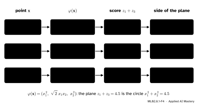
The quadratic map. A richer lift keeps all three products of two features:
A linear score on it, \({w_1 x_1^2 + \sqrt{2}\,w_2 x_1 x_2 + w_3 x_2^2 + b}\), is a general quadratic in \(x_1\) and \(x_2\) with no linear terms, so its boundaries are ellipses, hyperbolas or pairs of lines centred on the origin. The factor \(\sqrt{2}\) changes nothing about which boundaries are possible; the next lesson shows why it is there.
The cost. To catch every curve up to degree \(p\), the lift needs every monomial\({x_1^{a_1} x_2^{a_2} \cdots x_d^{a_d}}\) with \({a_1 + \dots + a_d \le p}\).
NoteResult: the size of a polynomial lift
On \(d\) features, the number of monomials of degree at most \(p\) is
\[
\binom{d + p}{p} .
\]
Derivation. Add a slack exponent \({a_0 = p - (a_1 + \dots + a_d)}\), so that each monomial matches exactly one list of \(d + 1\) whole numbers, each at least 0, adding up to \(p\). Write such a list as \(p\) stars split into \(d + 1\) groups by \(d\) bars: for \(d = 2\), \(p = 3\), the row *|**| means \({a_0 = 1}\), \({a_1 = 2}\), \({a_2 = 0}\), the monomial \(x_1^2\). Every row of \(p\) stars and \(d\) bars gives one list and every list one row. A row has \(p + d\) places, and choosing which \(p\) of them hold stars fixes it, so there are \({\binom{d + p}{p}}\) rows.
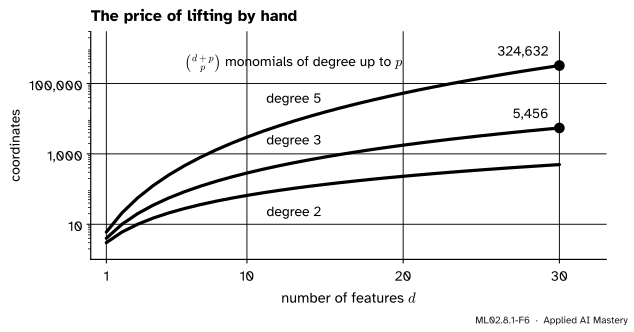
For two features and degree 2 that is \({\binom{4}{2} = 6}\): the monomials \(1\), \(x_1\), \(x_2\), \(x_1^2\), \({x_1 x_2}\), \(x_2^2\). For the 30 features of the breast cancer data and degree 3 it is
and degree 5 needs \({\binom{35}{5} = 324{,}632}\) columns: for its 569 rows, a table of about 185 million numbers.
ML02.8.1-F6
The number of coordinates of a polynomial lift against the number of features. Each step up in degree multiplies the count by roughly \(d/p\).
Worked example
Classify three ring points with the quadratic map and the rule \({z_1 + z_3 < 4.5}\).
Write \({\varphi(\vect{x}) = (z_1, z_2, z_3)}\). Since \({z_1 + z_3 = x_1^2 + x_2^2}\), the plane \({z_1 + z_3 = 4.5}\) in the lifted space is the circle of radius 2.12 again. Its weights are \({\vect{w} = (-1, 0, -1)}\) and \({b = 4.5}\), so the score is \({4.5 - z_1 - z_3}\).
The point \((1, 0)\). The products are \({1^2 = 1}\), \({\sqrt{2} \times 1 \times 0 = 0}\) and \({0^2 = 0}\), so \({\varphi = (1, 0, 0)}\). Then \({z_1 + z_3 = 1}\), below 4.5: class \(+1\).
The point \((-2, 2)\). Here \({(-2)^2 = 4}\), \({\sqrt{2} \times (-2) \times 2 = -4\sqrt{2} \approx -5.66}\) and \({2^2 = 4}\), so \({\varphi = (4, -4\sqrt{2}, 4)}\). Then \({z_1 + z_3 = 8}\), above 4.5: class \(-1\).
The point \((0, -3)\).\({\varphi = (0, 0, 9)}\) and \({z_1 + z_3 = 9}\): class \(-1\).
ML02.8.1-F4
Three points through the quadratic map. The middle coordinate is computed but not used by this rule; another rule could use it to tilt the ellipse.
One thing to notice: \({\varphi(1, 0) = \varphi(-1, 0) = (1, 0, 0)}\). Squaring forgets signs, so the map folds \(\vect{x}\) and \({-\vect{x}}\) onto the same lifted point. On the rings that does no harm, because each class is symmetric about the origin.
Code
First the lift by hand, then a linear classifier on raw and on lifted features.
lifted heights: [1. 1. 1. 1. 9. 9. 9. 9. 8. 8. 8. 8.]
the plane z = 4.5 is right on 12 of 12
phi of (1, 0), (-2, 2), (0, -3):
 [[ 1.     0.     0.   ]
 [ 4.    -5.657  4.   ]
 [ 0.    -0.     9.   ]]
raw features:    accuracy 0.6666666666666666  weights [0. 0.]
lifted features: accuracy 1.0  boundary at z = 4.43
On the raw features, logistic regression sets both weights to zero and keeps only the bias \({\ln(4/8) \approx -0.69}\), the log-odds of the class shares: every point is called \(-1\). On the lifted features it puts all its weight on \(z\) and draws its boundary at about \(z = 4.43\), between 1 and 8. It is not the plane at 4.5, because logistic regression does not look for the widest gap; ML02.7’s SVM does, and lesson 3 shows it finding 4.5 exactly.
scikit-learn builds polynomial lifts with PolynomialFeatures, and it can count them too.
from sklearn.pipeline import make_pipelinefrom sklearn.preprocessing import PolynomialFeaturesmodel = make_pipeline(PolynomialFeatures(degree=2), LogisticRegression(C=100)).fit(X, y)print("degree-2 features:", model[0].get_feature_names_out(), " accuracy", model.score(X, y))for d, p in [(2, 2), (30, 3), (30, 5)]: n_out = PolynomialFeatures(degree=p).fit(np.zeros((1, d))).n_output_features_print(f"d = {d:2d}, p = {p}: {n_out:,} columns, formula {math.comb(d + p, p):,}")
degree-2 features: ['1' 'x0' 'x1' 'x0^2' 'x0 x1' 'x1^2']  accuracy 1.0
d =  2, p = 2: 6 columns, formula 6
d = 30, p = 3: 5,456 columns, formula 5,456
d = 30, p = 5: 324,632 columns, formula 324,632
Explore
This module’s interactive, the kernel lift, lives in lesson 3. Its first half is this lesson’s picture: turn the lifted rings round, slide a flat plane up and down through them, and watch the circle it draws back in the plane grow and shrink.
Pitfalls
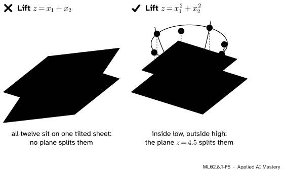
ML02.8.1-F5
Wrong beside right. Left: a new coordinate that is a straight combination of the old ones leaves every point on one flat sheet. Right: a curved coordinate separates the classes.
“More dimensions are what help, so any extra column will do.”
The extra column must be a non-linear function of the features. With \({z = x_1 + x_2}\), a plane in the lifted space scores \({w_1 x_1 + w_2 x_2 + w_3 (x_1 + x_2) + b}\), which is \({(w_1 + w_3) x_1 + (w_2 + w_3) x_2 + b}\): a line again. The lifted points all lie on one tilted sheet, and nothing has been gained.
“To be safe, lift with every monomial up to a high degree.”
The count \({\binom{d + p}{p}}\) explodes: 324,632 columns for degree 5 on 30 features. Memory and time grow with it, and so does the risk of overfitting, since a model with that many weights can fit noise (ML01.8). The next lesson removes the cost; regularisation and validation still have to handle the flexibility.
“The boundary is a circle, so the model is no longer linear and training is harder.”
The model is linear in its weights and in the lifted features; only its boundary, seen in the original features, is curved. Training solves exactly the problem it solved before, on a wider table, with the same guarantees.
Check yourself
Recall
1. Why can no line put the four inner ring points on one side and the eight outer ones on the other?
Show answer
For \((\pm 1, 0)\) the scores \({\pm w_1 + b}\) must both be positive, so their sum \(2b > 0\). For \((\pm 3, 0)\) the scores \({\pm 3w_1 + b}\) must both be negative, so \(2b < 0\). Both cannot hold.
2. What does the lifted coordinate \({z = x_1^2 + x_2^2}\) measure, and what heights do the rings get?
Show answer
The squared distance from the origin. The inner points get 1; the outer points get 9 (on the axes) or 8 (on the diagonals).
3. What curve in the original plane is the boundary of the rule “predict \(+1\) when \(z < 4.5\)”?
Show answer
The circle \({x_1^2 + x_2^2 = 4.5}\), of radius \({\sqrt{4.5} \approx 2.12}\), centred at the origin.
4. In what sense is a linear model on lifted features still linear?
Show answer
Its score \({\vect{w} \cdot \varphi(\vect{x}) + b}\) is linear in the weights and in the lifted features, so training is the same problem as before. Only its boundary in the original features is curved.
5. How many columns does a polynomial lift of degree 3 on 30 features have?
Show answer
\({\binom{33}{3} = 5{,}456}\), counting the constant 1.
Exercises
1.★ Lift the point \((1, 2)\) with \({\varphi(\vect{x}) = (x_1, x_2, x_1^2 + x_2^2)}\). On which side of the plane \(z = 4.5\) does it land, and what does that say about its place in the plane?
Show solution
\({\varphi(1, 2) = (1, 2, 1 + 4) = (1, 2, 5)}\). Its height 5 is above 4.5, so the rule calls it \(-1\). In the plane this says the point is outside the circle of radius 2.12: its distance from the origin is \({\sqrt{5} \approx 2.24}\).
2.★★ In the lifted space of exercise 1, take the plane \({z = 3 + 2x_2}\). What curve does it give in the plane? Does it separate the rings?
Show solution
The boundary is \({x_1^2 + x_2^2 = 3 + 2x_2}\). Move everything to the left and complete the square in \(x_2\):
It is the circle of radius 2 centred at \((0, 1)\). It does not separate the rings: \((0, -1)\) and \((0, 3)\) are both at distance exactly 2 from \((0, 1)\), so both lie on the boundary itself.
3.★★★ Show that the number of monomials of degree exactly\(q\) in \(d\) variables is \({\binom{d + q - 1}{q}}\). Check, for \(d = 2\) and \(p = 2\), that adding these counts over \(q = 0, 1, 2\) gives \({\binom{d + p}{p}}\).
Show solution
A monomial of degree exactly \(q\) is a list \({a_1, \dots, a_d}\) of whole numbers at least 0 that add up to \(q\), with no slack. Write it as \(q\) stars split into \(d\) groups by \({d - 1}\) bars. A row has \({q + d - 1}\) places, and choosing which \(q\) hold stars fixes it, so the count is \({\binom{d + q - 1}{q}}\).
For \(d = 2\): degree 0 gives \({\binom{1}{0} = 1}\), degree 1 gives \({\binom{2}{1} = 2}\) and degree 2 gives \({\binom{3}{2} = 3}\). The total is \({1 + 2 + 3 = 6 = \binom{4}{2}}\), matching the six columns 1, \(x_1\), \(x_2\), \(x_1^2\), \({x_1 x_2}\), \(x_2^2\).
Summary card
Do not bend the model: lift the data until a straight cut works.
ML02.8.1-F1
A flat plane in the lift is a circle below.
Feature map.\({\varphi : \R^d \to \R^D}\); the model scores \({\vect{w} \cdot \varphi(\vect{x}) + b}\).
The rings.\({z = x_1^2 + x_2^2}\) gives 1 inside and 8 or 9 outside; \(z = 4.5\) splits them.
Planes become circles. With \((x_1, x_2, z)\), the boundary is a circle centred at \({(-w_1/2w_3,\; -w_2/2w_3)}\).
The cost. A polynomial lift of degree \(p\) on \(d\) features has \({\binom{d + p}{p}}\) columns.
Sources and next steps
Sources. Each was opened and checked against this lesson on 15 November 2026.
Gareth James, Daniela Witten, Trevor Hastie, Robert Tibshirani and Jonathan Taylor, An Introduction to Statistical Learning with Applications in Python (free PDF from the authors), Section 9.3.1. Enlarges the feature space with the squares of the predictors (equation 9.16), notes that the boundary is linear in the enlarged space but quadratic in the original one, and warns that with many ways to enlarge the space “we could end up with a huge number of features” and computations would become unmanageable.
Tengyu Ma and Andrew Ng, CS229 Lecture Notes, Stanford University, Sections 5.1 and 5.4. Defines feature maps and states that the polynomial kernel of degree \(k\) corresponds to a feature map into a space of dimension \({\binom{d + k}{k}}\), all monomials up to order \(k\).
scikit-learn 1.9 API reference, PolynomialFeatures. Gives the degree-2 features of \({[a, b]}\) as \({[1, a, b, a^2, ab, b^2]}\), the attribute n_output_features_, and the warning that the number of output features grows polynomially in the number of inputs and exponentially in the degree, and that high degrees can overfit.