When two classes can be split by a straight line, infinitely many lines do it. The maximum-margin line is the one furthest from the closest points: the centre of the widest street between the classes. Derive the distance to a line and find the street for six points by hand.
ML02.7.1L2 Intermediate25 minIn review (what this means)
The maths and code on this page are checked by automated tests on every change, but an independent reader has not signed it off yet. Spot a mistake or a confusing step? Tell us.
Define the margin of a separating line and explain why the maximum-margin line is a sensible choice among all separating lines.
Derive the distance from a point to the hyperplane w . x + b = 0 by projecting onto w.
Explain why (w, b) can be rescaled so that the closest points have |w . x + b| = 1, and show that the street is then 2/||w|| wide.
Find the maximum-margin line of a small symmetric data set by hand and check it with code.
The question
Six points in the plane, three of each class, and a gap between them. A straight line can split them without a single mistake, but so can a vertical line, a horizontal one and infinitely many others. All of them score 100 percent on the training data. Which one should a classifier choose, and why should the answer depend on only three of the six points?
Intuition
Logistic regression (ML01.6) answers with probabilities. Here we answer with geometry. Think of the line as the centre of a street that runs between the two classes, with no point allowed on the street. Some separating lines leave only a narrow lane; others leave room for a wide road. Choose the line whose street is widest.
ML02.7.1-F1
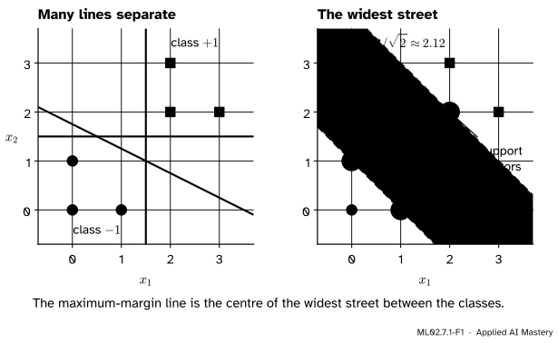
Left: three of the infinitely many lines that separate the six points. Right: the widest street. Its centre line is the maximum-margin line, and the three points on its edges are the support vectors.
The picture already shows the two facts this module is built on. First, the widest street is pinned by a few points that touch its edges, here \((1, 0)\), \((0, 1)\) and \((2, 2)\). They are called support vectors: move any of them and the street moves. Second, the other three points do not matter at all. Slide \((0, 0)\) or \((3, 2)\) around, without letting it onto the street, and nothing changes.
Why prefer a wide street? A new point is measured with some noise. If the line passes close to a training point, a small wobble in a similar new point can carry it across the line. A wide street leaves the most room for such wobbles on both sides. This classifier, built on the widest street, is the support vector machine (SVM). It made a splash when it was introduced in the mid-1990s (ISL, Section 9.5), and a linear SVM is still a strong, fast baseline for many classification tasks.
Build it up
Step 1. Every separating line has a margin. For a line that separates the classes, measure the distance from each point to the line. The smallest of these distances is the margin of the line. It is the half-width of the widest street that can be centred on that line.
ML02.7.1-F2
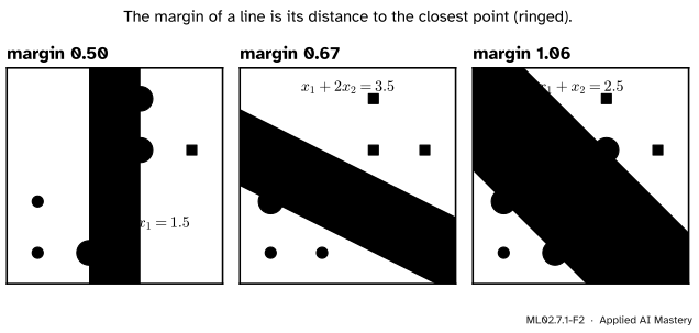
Three separating lines and their margins. The vertical line comes within \(0.50\) of three points, the slanted line within \(0.67\) of \((0, 1)\), and the diagonal line keeps a distance of \(1.06\) from everything.
Step 2. Compare the lines by their margins. The three lines of the figure have margins \(0.50\), \(0.67\) and \(1.06\). The maximum-margin line is the separating line with the largest margin. To find it we need a formula for the distance from a point to a line.
Step 3. Name the line by a weight vector. As in ML01.6.4, a line is the set of points where a score is zero:
The weight vector\(\vect{w}\) is at a right angle to the line, and the classifier predicts \({+1}\) where \({f(\vect{x}) > 0}\) and \({-1}\) where \({f(\vect{x}) < 0}\). With labels \({y_i \in \{-1, +1\}}\), a point is on its correct side exactly when \({y_i f(\vect{x}_i) > 0}\). That is why SVMs use the labels \(-1\) and \(+1\) instead of \(0\) and \(1\).
Step 4. The score is not the distance. The pairs \((\vect{w}, b)\) and \({(2\vect{w}, 2b)}\) describe the same line, yet the second doubles every score. So the score measures distance only after we divide by something that also doubles: the length \(\norm{\vect{w}}\).
The formal statement
The distance from a point to a hyperplane. In \(d\) dimensions the set \({\vect{w} \cdot \vect{x} + b = 0}\) is a hyperplane: a line when \({d = 2}\), a plane when \({d = 3}\).
ML02.7.1-F3
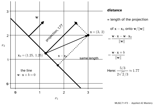
The distance from \(\vect{x}\) to the line is the length of the projection of \({\vect{x} - \vect{x}_0}\) onto the direction of \(\vect{w}\), for any point \(\vect{x}_0\) on the line.
Take any point \(\vect{x}_0\) on the hyperplane, so that \({\vect{w} \cdot \vect{x}_0 = -b}\). The shortest path from \(\vect{x}\) to the hyperplane runs at a right angle to it, which is along \(\vect{w}\). So the distance is the length of the projection of \({\vect{x} - \vect{x}_0}\) onto the unit vector \({\vect{w} / \norm{\vect{w}}}\) (M02.3.4):
The last step replaces \({\vect{w} \cdot \vect{x}_0}\) by \(-b\). The sign says which side \(\vect{x}\) is on, and the distance itself is \({\abs{\vect{w} \cdot \vect{x} + b} / \norm{\vect{w}}}\). The choice of \(\vect{x}_0\) has dropped out, as it must.
The margin and the problem. For a line that separates the data, every \({y_i (\vect{w} \cdot \vect{x}_i + b)}\) is positive and equals the score’s size, so
The maximum-margin line maximises this over all \(\vect{w}\) and \(b\).
Fixing the scale. Multiplying \(\vect{w}\) and \(b\) by any \({c > 0}\) leaves the line and the margin unchanged: the \(c\) cancels between top and bottom. So we may choose the scale. Choose it so that the closest points have score exactly \(\pm 1\):
Then the margin is \({1 / \norm{\vect{w}}}\). The two edges of the street are the lines \({\vect{w} \cdot \vect{x} + b = 1}\) and \({\vect{w} \cdot \vect{x} + b = -1}\), one margin either side of the centre, and the street is
\[
\text{width} = \frac{2}{\norm{\vect{w}}}
\]
wide. Every point satisfies \({y_i (\vect{w} \cdot \vect{x}_i + b) \ge 1}\): none is on the street. A wide street means a short \(\vect{w}\). Lesson 2 turns this into an optimisation problem.
Go deeper: why the widest street is unique
With the scale fixed, the widest street minimises \(\norm{\vect{w}}^2\) over all \((\vect{w}, b)\) with every \({y_i (\vect{w} \cdot \vect{x}_i + b) \ge 1}\). Suppose two different weight vectors \(\vect{w}_1\) and \(\vect{w}_2\) both reached the smallest value \(m\). Their average, with the average bias, satisfies every constraint too, because each constraint is linear. But for \({\vect{w}_1 \neq \vect{w}_2}\),
which contradicts \(m\) being the smallest. So \(\vect{w}\) is unique. The bias is then fixed too: the closest points on each side must have scores \(-1\) and \(+1\).
Worked example
The six points. Class \(-1\) at \((0, 0)\), \((1, 0)\), \((0, 1)\); class \(+1\) at \((2, 2)\), \((3, 2)\), \((2, 3)\).
Symmetry gives the direction. Swapping the two coordinates maps each class onto itself. If \({(w_1, w_2)}\) with bias \(b\) gave the widest street, then \({(w_2, w_1)}\) with the same \(b\) would give a street just as wide, and the widest street is unique. So \({w_1 = w_2}\): write \({\vect{w} = (a, a)}\). The score is then \({a\,(x_1 + x_2) + b}\), which depends on the point only through \({s = x_1 + x_2}\).
ML02.7.1-F4
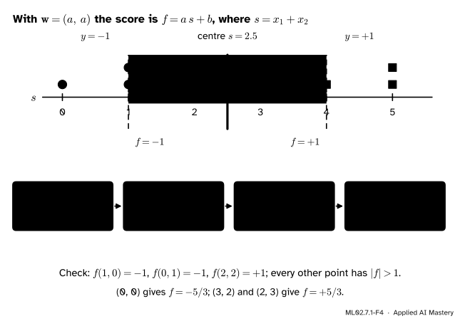
The six points seen through \({s = x_1 + x_2}\). The closest pair across the gap is \({s = 1}\) and \({s = 4}\); setting their scores to \(-1\) and \(+1\) fixes \(a\) and \(b\).
The closest points fix the scale. The \(s\) values of class \(-1\) are \(0, 1, 1\); those of class \({+1}\) are \(4, 5, 5\). The closest points across the gap have \({s = 1}\) and \({s = 4}\), so their scores must be \(-1\) and \(+1\):
\[
\begin{aligned}
a \cdot 1 + b &= -1, \\
a \cdot 4 + b &= +1 .
\end{aligned}
\]
Subtracting the first line from the second gives \({3a = 2}\), so \({a = 2/3}\), and then \({b = -1 - 2/3 = -5/3}\):
and the margin is half of it, \({3/(2\sqrt{2}) \approx 1.06}\), the value in the figure of Step 1.
Check. The scores are \({f(1, 0) = f(0, 1) = -1}\) and \({f(2, 2) = +1}\): three points on the edges, the support vectors. The others have \({f(0, 0) = -5/3}\) and \({f(3, 2) = f(2, 3) = +5/3}\), safely off the street. Note that \({(1, 0)}\) and \({(0, 1)}\) both count: with only \({(2, 2)}\) on the \(+1\) side, two points on the other side are needed to stop the street from turning.
Code
From scratch first. In the plane a direction is an angle \(\theta\). For the unit vector \({\vect{u} = (\cos\theta, \sin\theta)}\), the gap between the classes along \(\vect{u}\) is the smallest \({\vect{u} \cdot \vect{x}}\) of class \(+1\) minus the largest of class \(-1\). The widest street is the direction with the largest gap, so we try 3,601 angles.
import numpy as npX = np.array([[0, 0], [1, 0], [0, 1], [2, 2], [3, 2], [2, 3]], dtype=float)y = np.array([-1, -1, -1, 1, 1, 1])def margin(w, b):"""Distance from the line w . x + b = 0 to the closest point."""return np.min(np.abs(X @ w + b)) / np.linalg.norm(w)for w, b in [((1, 0), -1.5), ((1, 2), -3.5), ((1, 1), -2.5)]:print(f"line {w}, b = {b}: margin {margin(np.array(w, float), b):.2f}")theta = np.linspace(0, np.pi, 3601) # angles in steps of 0.05 degreesU = np.column_stack([np.cos(theta), np.sin(theta)])proj = X @ U.T # one column per directiongap = proj[y ==1].min(axis=0) - proj[y ==-1].max(axis=0)best = gap.argmax()print(f"widest street at {np.degrees(theta[best]):.1f} degrees, width {gap[best]:.4f}")print("3 / sqrt(2) =", round(3/ np.sqrt(2), 4))
line (1, 0), b = -1.5: margin 0.50
line (1, 2), b = -3.5: margin 0.67
line (1, 1), b = -2.5: margin 1.06
widest street at 45.0 degrees, width 2.1213
3 / sqrt(2) = 2.1213
Turn the best direction into \(\vect{w}\) and \(b\) with the scale rule: the gap must equal \({2 / \norm{\vect{w}}}\), and the centre of the gap must score zero.
u = U[best]w =2/ gap[best] * u # length 2 / widthlow, high = proj[y ==-1, best].max(), proj[y ==1, best].min()b =-np.linalg.norm(w) * (low + high) /2# the centre of the gap scores zeroscores = X @ w + bprint("w =", np.round(w, 4), " b =", round(b, 4))print("y * score:", np.round(y * scores, 4))print("support vectors:", X[np.isclose(y * scores, 1)].tolist())
w = [0.6667 0.6667]  b = -1.6667
y * score: [1.6667 1.     1.     1.     1.6667 1.6667]
support vectors: [[1.0, 0.0], [0.0, 1.0], [2.0, 2.0]]
scikit-learn’s SVC with a linear kernel solves the same problem. A very large C asks for no point on the street (lesson 3 explains C); tol makes the solver run to high accuracy.
w = [0.6667 0.6667]  b = -1.6667
support vectors: [[1.0, 0.0], [0.0, 1.0], [2.0, 2.0]]
width: 2.1213
The angle scan works only in two dimensions. With 30 features there is no list of angles to try, which is why the next lesson turns the widest street into a problem that a solver can handle.
Explore
The margin explorer of this module is in lesson 3. Press Six points and Hard margin: the street of this lesson appears with its three ringed support vectors and the width \(2.12\). Drag \((3, 2)\) around the \(+1\) side: nothing moves until the point reaches the edge of the street. Then drag \((2, 2)\) and watch the whole street turn.
Pitfalls
ML02.7.1-F5
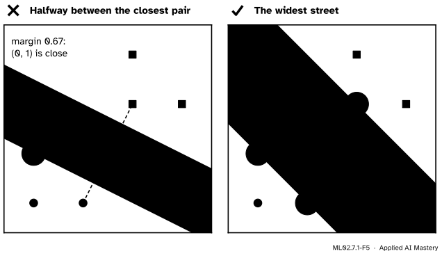
Wrong beside right. The line halfway between the closest pair of opposite points ignores \((0, 1)\), which ends up only \(0.67\) from it. The widest street keeps \(1.06\) from every point.
“The street runs halfway between the two closest points of opposite classes.”
A closest opposite pair is \({(1, 0)}\) and \({(2, 2)}\), at distance \({\sqrt{5} \approx 2.24}\) (the pair \({(0, 1)}\) and \({(2, 2)}\) ties with it). The line halfway between them, at a right angle to the segment, has margin only \(0.67\), and the true width \(2.12\) is less than \(2.24\). The street is pinned by the closest groups: here the whole segment from \({(1, 0)}\) to \({(0, 1)}\) faces the point \({(2, 2)}\). In general the width is the distance between the convex hulls of the two classes.
“The score \(\vect{w} \cdot \vect{x} + b\) is the distance to the line.”
Only when \({\norm{\vect{w}} = 1}\). The point \({(3, 2)}\) has score \({5/3 \approx 1.67}\) but distance \({(5/3) / (2\sqrt{2}/3) \approx 1.77}\). Doubling \(\vect{w}\) and \(b\) doubles every score and moves nothing. Divide by \(\norm{\vect{w}}\) before you call a score a distance.
“Perfect training accuracy settles it.”
Every line in the first figure has perfect training accuracy, so accuracy cannot choose between them. Logistic regression does not settle it either: on separable data its loss keeps falling as \(\vect{w}\) grows, so without a penalty the weights never stop growing (ML01.6.3). The margin is an extra principle, and the next lessons show it makes a well-posed problem with one answer.
Frontier note: gradient descent finds the widest street by itself
Soudry and co-authors (2018) studied gradient descent on unregularised logistic regression with separable data and a linear model with no separate bias term. The weights grow without limit, but their direction converges to the direction of the hard-margin SVM solution, and it does so very slowly, only logarithmically in the number of steps. This “implicit bias” towards large margins is one of the ideas used to explain why trained neural networks generalise.
Check yourself
Recall
1. What is the margin of a separating line?
Show answer
The distance from the line to the closest training point. It is the half-width of the widest street centred on that line.
2. Write the distance from a point \(\vect{x}\) to the hyperplane \({\vect{w} \cdot \vect{x} + b = 0}\).
Show answer
\({\abs{\vect{w} \cdot \vect{x} + b} / \norm{\vect{w}}}\), found by projecting \({\vect{x} - \vect{x}_0}\) onto \({\vect{w} / \norm{\vect{w}}}\) for a point \(\vect{x}_0\) on the hyperplane.
3. Why may we rescale \(\vect{w}\) and \(b\) so that the closest points score \(\pm 1\)?
Show answer
Because \({(c\vect{w}, cb)}\) with \({c > 0}\) is the same line with the same margin. Fixing the scale this way makes the margin \({1 / \norm{\vect{w}}}\) and the width \({2 / \norm{\vect{w}}}\).
4. For the six points, give \(\vect{w}\), \(b\), the width and the support vectors.
Show answer
\({\vect{w} = (2/3, 2/3)}\), \({b = -5/3}\), width \({3/\sqrt{2} \approx 2.12}\), support vectors \({(1, 0)}\), \({(0, 1)}\) and \({(2, 2)}\).
5. What happens to the maximum-margin line if you move \({(0, 0)}\) to \({(-1, 0)}\)?
Show answer
Nothing. \({(0, 0)}\) is not a support vector, and \({(-1, 0)}\) is still off the street (its score is \(-7/3\)), so the widest street is unchanged.
Exercises
1.★ Find the distance from \({(2, 3)}\) to the line \({3x_1 + 4x_2 - 6 = 0}\), and say on which side of the line it lies.
Show solution
The score is \({3 \cdot 2 + 4 \cdot 3 - 6 = 12}\) and \({\norm{\vect{w}} = \sqrt{9 + 16} = 5}\), so the distance is \({12 / 5 = 2.4}\). The score is positive, so the point lies on the side that \(\vect{w} = (3, 4)\) points to.
2.★★ One feature. Class \(-1\) at \({x = 1, 2}\) and class \(+1\) at \({x = 5, 7}\). Find the maximum-margin rule \({f(x) = wx + b}\), its width and its support vectors.
Show solution
The closest pair across the gap is \({x = 2}\) and \({x = 5}\). Setting their scores to \(-1\) and \(+1\):
\[
\begin{aligned}
2w + b &= -1, \\
5w + b &= +1 .
\end{aligned}
\]
Subtracting gives \({3w = 2}\), so \({w = 2/3}\) and \({b = -1 - 4/3 = -7/3}\). The boundary is \({x = 3.5}\), the width is \({2 / w = 3}\), the gap from \(2\) to \(5\), and the support vectors are \({x = 2}\) and \({x = 5}\).
3.★★★ Add a seventh point to the six: class \(+1\) at \({(1.5, 1.5)}\). Find the new maximum-margin line and width.
Show solution
The swap symmetry still holds, so \({\vect{w} = (a, a)}\) and only \({s = x_1 + x_2}\) matters. The new point has \({s = 3}\), closer to class \(-1\) than \({(2, 2)}\) was. The closest pair across the gap is now \({s = 1}\) and \({s = 3}\):
\[
\begin{aligned}
a + b &= -1, \\
3a + b &= +1 ,
\end{aligned}
\]
so \({2a = 2}\), \({a = 1}\), \({b = -2}\). The centre line is \({x_1 + x_2 = 2}\) and the width is \({2 / \norm{\vect{w}} = 2/\sqrt{2} = \sqrt{2} \approx 1.41}\). The support vectors are \({(1, 0)}\), \({(0, 1)}\) and \({(1.5, 1.5)}\); \({(2, 2)}\) now has score \({+2}\) and no longer touches the street.
Summary card
The maximum-margin line is the centre of the widest street.
ML02.7.1-F1
Few points pin the street.
Distance to a hyperplane.\({\abs{\vect{w} \cdot \vect{x} + b} / \norm{\vect{w}}}\).
Scale rule. Closest points score \(\pm 1\), so every \({y_i (\vect{w} \cdot \vect{x}_i + b) \ge 1}\).
Width.\({2 / \norm{\vect{w}}}\): a wide street is a short \(\vect{w}\).
Six points.\({\vect{w} = (2/3, 2/3)}\), \({b = -5/3}\), width \({3/\sqrt{2}}\), support vectors \({(1, 0)}\), \({(0, 1)}\), \({(2, 2)}\).
Sources and next steps
Sources. Each was opened and checked against this lesson on 15 November 2026.
Gareth James, Daniela Witten, Trevor Hastie and Robert Tibshirani, An Introduction to Statistical Learning, 2nd edition (corrected June 2023), free PDF from the authors. Section 9.1.3 defines the margin as the smallest perpendicular distance to the hyperplane, the maximal margin hyperplane as the separating hyperplane with the largest margin, and support vectors as the points that “support” it; it notes that moving any other point does not change the hyperplane. Section 9.1.4 states the problem as equations (9.9) to (9.11).
Trevor Hastie, Robert Tibshirani and Jerome Friedman, The Elements of Statistical Learning, 2nd edition, Section 4.5.2: the problem (4.45), the rescaling that sets the margin to \({1/\norm{\vect{w}}}\) in (4.46) to (4.48), and the remark that the solution is unique.
Kilian Weinberger, Lecture 9: SVM, Cornell CS4780, Fall 2018. Derives the distance \({\abs{\vect{w}\T\vect{x} + b} / \norm{\vect{w}}_2}\) by projection and fixes the scale so that the closest point has \({\abs{\vect{w}\T\vect{x} + b} = 1}\).
Daniel Soudry, Elad Hoffer, Mor Shpigel Nacson, Suriya Gunasekar and Nathan Srebro, The Implicit Bias of Gradient Descent on Separable Data, arXiv:1710.10345. The abstract states that, for unregularised logistic regression on separable data, the predictor converges to the direction of the hard-margin SVM solution, and that the convergence is only logarithmic.
Next.ML02.7.2 The hard-margin problem and its dual writes the widest street as “minimise \({\tfrac{1}{2}\norm{\vect{w}}^2}\)” and solves it with Lagrange multipliers, which recover the support vectors and their weights.