XGBoost adds a price on leaves to the boosting loss and replaces each loss by its parabola. Then every leaf is a parabola in its weight, and one formula, G squared over H plus lambda, gives the leaf weight, the score of a tree and the gain of a split.
ML02.5.1L2 Intermediate30 minIn review (what this means)
The maths and code on this page are checked by automated tests on every change, but an independent reader has not signed it off yet. Spot a mistake or a confusing step? Tell us.
Write XGBoost’s regularised objective for one boosting stage and say what gamma and lambda each charge for.
Derive the leaf weight -G/(H + lambda), the structure score and the split gain from a second-order expansion of the loss.
Compute the gain of every threshold of a small dataset by hand, with and without lambda and gamma, and check that lambda = 0 with the squared loss gives back ordinary gradient boosting.
Build a second-order split finder in NumPy, match it against HistGradientBoostingRegressor, and explain what min_child_weight bounds.
The question
Gradient boosting grows each tree by squared error on the pseudo-residuals and only afterwards fixes the leaf values with the true loss. Two criteria for one tree. XGBoost, the library that made boosting the default for tables of data, uses a single number for both jobs, and puts a price on every leaf while it is at it. What is that number, and why does it look like \({G^2/(H + \lambda)}\)?
Intuition
At each stage, boosting adds a tree \(f\) to the current model \(F\). Every leaf of the tree moves the prediction of all its points by the same amount, the leaf’s weight\(w\). XGBoost asks: how far does the loss fall if this leaf moves by \(w\)? It answers with a parabola in \(w\).
ML02.5.1-F1
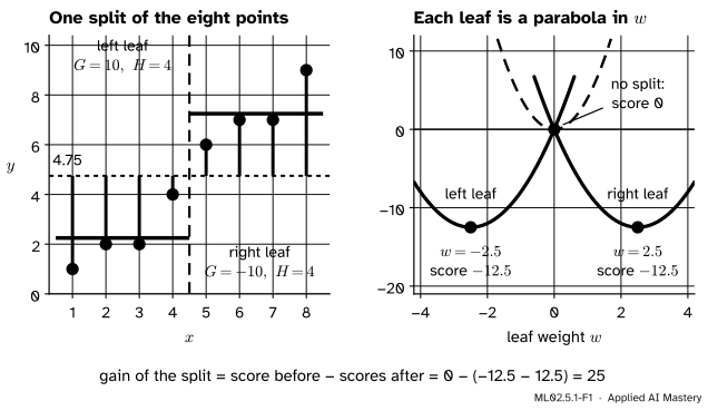
The first stage on the eight points. Left: the split \(x \le 4.5\) sorts the points into two leaves. Right: each leaf’s share of the objective is a parabola in its weight. The bottoms give the leaf weights \(\mp 2.5\), and how much lower the two bottoms reach than the single one is the gain of the split, \(25\).
The picture holds the whole lesson. For each leaf, add up the slopes of the points’ losses, \(G\), and their curvatures, \(H\). The leaf’s parabola has its bottom at \(w = -G/H\) and its lowest value at \(-\tfrac12 G^2/H\), the leaf’s score. A split is good when the two new leaves reach lower than the old leaf did: that difference is the gain. XGBoost adds two prices. A charge \(\lambda\) widens every parabola, and a fee \(\gamma\) is paid for every leaf.
Build it up
Step 1. A tree is a list of leaf weights. A tree with \(T\) leaves sends each input to one leaf \(j\) and outputs that leaf’s weight \(w_j\). Write \(I_j\) for the set of training points that land in leaf \(j\). Then \({f(x_i)} = w_j\) for every \(i\) in \(I_j\).
Step 2. A price on the tree. XGBoost charges \(\gamma\) for every leaf and \(\tfrac12\lambda w_j^2\) for every weight, the ridge penalty of ML01.9 put on the leaves: \({\Omega(f)} = \gamma T + \tfrac12 \lambda \sum_j w_j^2\).
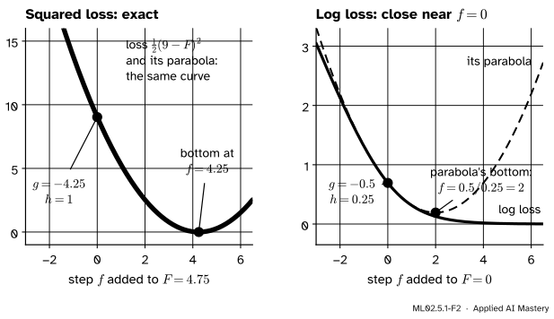
Step 3. Replace each loss by its parabola. Near the current prediction \(F\), a smooth loss looks like a parabola in the step \(f\) that is added. It has the loss’s slope \(\cgrad{g_i}\) and curvature \(h_i\) at \(F\):
The second-order expansion. Left: for the squared loss \({\tfrac12(y - F)^2}\) the parabola is the loss, with \(h = 1\) everywhere. Right: for the log loss it agrees at \(f = 0\) in value, slope and curvature, and drifts away further out.
For the squared loss \(\ell = {\tfrac12(y - F)^2}\), \(g_i = F - y_i\) (minus the residual) and \(h_i = 1\). For the log loss of ML02.4.3, with \(p_i\) the predicted probability, \(g_i = p_i - y_i\) and \(h_i = {p_i(1 - p_i)}\).
Step 4. Collect by leaves. All points of leaf \(j\) share the step \(w_j\). So their slopes add up to \(G_j = \sum_{i \in I_j} g_i\) and their curvatures to \(H_j = \sum_{i \in I_j} h_i\), and the leaf contributes the single parabola \(G_j w_j + {\tfrac12 (H_j + \lambda) w_j^2}\).
Step 5. Go to the bottom. Each parabola has its own weight, so each leaf can be minimised on its own. The bottom gives the weight; its height scores the leaf.
The formal statement
NoteDefinition: the regularised objective of stage \(m\)
Given the model \(F_{m-1}\), choose the tree \(f\) to minimise
then set \(F_m = F_{m-1} + \nu f\), where \(\nu\) is the learning rate.
NoteResult: leaf weight, structure score and split gain
With \(G_j\) and \(H_j\) the sums of \(g_i\) and \(h_i\) over leaf \(j\), the best weights are \(\cmodel{w_j} = {-G_j/(H_j + \lambda)}\) and the best value of the approximate objective is the structure score
The first sum does not depend on \(f\), so drop it. Call what is left \(\tilde{\mathcal{L}}\).
Collect. Every point lies in exactly one leaf, so a sum over points is a sum over leaves of sums over their points. Inside leaf \(j\), \({f(x_i)} = w_j\):
Minimise. Term \(j\) contains \(w_j\) and no other weight, so each term is minimised on its own. Its derivative is \(G_j + {(H_j + \lambda) w_j}\), which is zero at
\[
w_j = -\frac{G_j}{H_j + \lambda} .
\]
The second derivative is \(H_j + \lambda\). For a convex loss every \(h_i \ge 0\), so this is positive whenever \(\lambda > 0\) or \(H_j > 0\): the point is a minimum.
Summing over the leaves and adding \(\gamma T\) gives the structure score.
The gain. Split one leaf with sums \(G = G_L + G_R\) and \(H = H_L + H_R\). Before, that leaf adds \({-\tfrac12 G^2/(H + \lambda)}\) and one fee \(\gamma\) to the score. After, the two new leaves add \({-\tfrac12 G_L^2/(H_L + \lambda)} - {\tfrac12 G_R^2/(H_R + \lambda)}\) and two fees. The other leaves do not change. The gain is the score before minus the score after, which is the formula in the box. A split is made only when its gain is positive, so \(\gamma\) is the least gain a split must earn.
ML02.5.1-F3
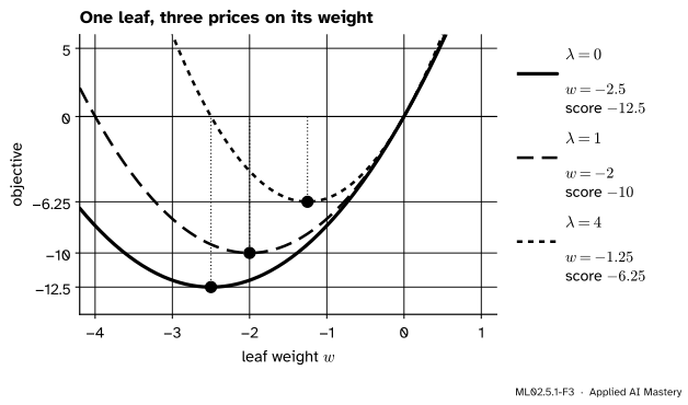
What \(\lambda\) does to one leaf, \(G = 10\) and \(H = 4\). It widens the parabola, so the bottom moves towards \(w = 0\) and rises: \(\lambda = 0, 1, 4\) give \(w = -2.5, -2, -1.25\).
Two checks. With the squared loss, \(h_i = 1\), so \(H_j\) is the number of points in the leaf and, with \(\lambda = 0\), \(w_j = -G_j/H_j\) is the mean residual of the leaf: the leaf value of ML02.4.1. With the log loss and \(\lambda = 0\), \(w_j = {\sum (y_i - p_i) / \sum p_i(1 - p_i)}\): the Newton leaf of ML02.4.3. XGBoost is gradient boosting that chooses the tree by the same second-order score it uses for the leaves.
Hessian floor. The setting min_child_weight allows a split only if \({H_L \ge m}\) and \({H_R \ge m}\) for a chosen \(m\). With the squared loss this is a minimum number of points per leaf. With the log loss it is not: a point with \(p = 0.98\) has \(h = 0.0196\).
Go deeper: the expansion as a weighted least-squares fit
The last term does not depend on \(f\). So each stage fits the tree by weighted least squares to the targets \(-g_i/h_i\), with weights \(h_i\). Chen and Guestrin use this view in their Section 3.3: when candidate thresholds are proposed from quantiles of a feature, each point should count with its weight \(h_i\), which led to their weighted quantile sketch.
Worked example
The eight points, \(x = 1, \dots, 8\) and \(y = {(1, 2, 2, 4, 6, 7, 7, 9)}\), with the squared loss. The first prediction is the mean, \(4.75\), so \(g_i = 4.75 - y_i\):
and every \(h_i = 1\). In total \(G = 0\) and \(H = 8\).
Threshold 4.5, \(\lambda = 0\). The left leaf holds the first four points: \(G_L = 3.75 + 2.75 + 2.75 + 0.75 = 10\) and \(H_L = 4\). The right leaf has \(G_R = -10\), \(H_R = 4\).
The weights are \(w_L = -10/4 = -2.5\) and \(w_R = 2.5\), so the new predictions are \(4.75 - 2.5 = 2.25\) and \(4.75 + 2.5 = 7.25\): the stump of ML02.4.1.
The predictions become \(2.75\) and \(6.75\): each leaf moves only four fifths of the way to its mean.
ML02.5.1-F4
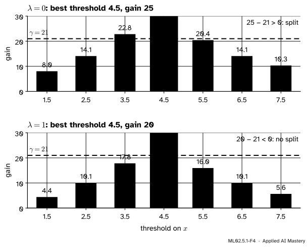
The trace of the first stage: the gain of every threshold. Both values of \(\lambda\) choose \(4.5\). With a fee of \(\gamma = 21\) per extra leaf, the split pays for itself only when \(\lambda = 0\).
The fee \(\gamma\). Take \(\gamma = 21\). With \(\lambda = 0\) the best gain is \(25 - 21 = 4 > 0\), and the split is made. With \(\lambda = 1\) it is \(20 - 21 = -1\), and the tree stays a single leaf. (XGBoost’s code measures gains without the \(\tfrac12\), so there the same fee is gamma=42; ML02.5.4 returns to this.)
Later stages. With \(\lambda = 0\) the second and third stages split at \(7.5\) and \(1.5\) and the training error falls to \(0.75\) and \(0.6071\), as in ML02.4.1. Add min_child_weight\(= 3\) and the second stage may no longer cut off the single point \(x = 8\); it splits at \(3.5\) instead, with gain \(0.8167\).
Code
The split finder sorts the points once and sweeps a cut from left to right, keeping running sums of \(g\) and \(h\): the sorted search of ML02.1.3 with a new score.
import numpy as npx = np.arange(1.0, 9.0)y = np.array([1.0, 2.0, 2.0, 4.0, 6.0, 7.0, 7.0, 9.0])def leaf_weight(G, H, lam):return-G / (H + lam)def split_gain(GL, HL, GR, HR, lam, gamma=0.0): G, H = GL + GR, HL + HRreturn0.5* (GL**2/ (HL + lam) + GR**2/ (HR + lam) - G**2/ (H + lam)) - gammadef best_split(x, g, h, lam=0.0, gamma=0.0, min_child_weight=0.0):"""The best threshold on one feature, and its gain.""" order = np.argsort(x) xs, gs, hs = x[order], g[order], h[order] GL, HL = np.cumsum(gs)[:-1], np.cumsum(hs)[:-1] # left of each cut GR, HR = gs.sum() - GL, hs.sum() - HL # right of it gains = split_gain(GL, HL, GR, HR, lam, gamma) allowed = (xs[1:] > xs[:-1]) & (HL >= min_child_weight) & (HR >= min_child_weight) gains = np.where(allowed, gains, -np.inf) k =int(np.argmax(gains))returnfloat((xs[k] + xs[k +1]) /2), float(gains[k])g, h = y.mean() - y, np.ones_like(y) # squared loss at F = 4.75for lam in (0.0, 1.0):print(f"lam = {lam}: best split {best_split(x, g, h, lam)}")print("gamma = 21:", best_split(x, g, h, 0.0, 21.0)[1], best_split(x, g, h, 1.0, 21.0)[1])
lam = 0.0: best split (4.5, 25.0)
lam = 1.0: best split (4.5, 20.0)
gamma = 21: 4.0 -1.0
Now boosting with stumps: one split per stage, leaf weights from the formula.
def boost(x, y, lam=0.0, stages=3, min_child_weight=0.0, nu=1.0): F = np.full(len(y), y.mean()) trace = []for _ inrange(stages): g, h = F - y, np.ones_like(y) threshold, gain = best_split(x, g, h, lam, 0.0, min_child_weight) left = x <= threshold w_left = leaf_weight(g[left].sum(), h[left].sum(), lam) w_right = leaf_weight(g[~left].sum(), h[~left].sum(), lam) F = F + nu * np.where(left, w_left, w_right) trace.append((float(threshold), round(float(np.mean((y - F) **2)), 4)))return F, traceprint("lam = 0:", boost(x, y, 0.0)[1])print("lam = 1:", boost(x, y, 1.0)[1])print("lam = 0, min_child_weight = 3:", boost(x, y, 0.0, min_child_weight=3)[1])
With \(\lambda = 1\) the second stage splits at \(3.5\), not \(7.5\): the one-point leaf at \(x = 8\) would keep only half of its step, \({-G/(1 + 1)}\), so cutting it off is worth less. Its training error after three stages happens to be lower here; that is the luck of greedy choices, not a rule.
scikit-learn’s HistGradientBoostingRegressor grows its trees with the same formulas; l2_regularization is \(\lambda\). A stump is a tree with two leaves.
from sklearn.ensemble import HistGradientBoostingRegressorfor lam in (0.0, 1.0): model = HistGradientBoostingRegressor(max_iter=3, learning_rate=1.0, max_leaf_nodes=2, min_samples_leaf=1, l2_regularization=lam, early_stopping=False).fit(x.reshape(-1, 1), y) ours = boost(x, y, lam)[0]print(f"lam = {lam}: library matches ours: {np.allclose(model.predict(x.reshape(-1, 1)), ours)}")
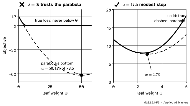
Last, the log loss, where a tiny Hessian makes a huge step. Three points with \(y = 1\) that the model gives \(p = 0.02\) share a leaf:
p = np.full(3, 0.02)G, H = np.sum(p -1), np.sum(p * (1- p))loss_now = np.sum(np.log(1/ p))print(f"G = {G:.2f}, H = {H:.4f}, loss now {loss_now:.2f}")for lam in (0.0, 1.0): w = leaf_weight(G, H, lam)print(f"lam = {lam}: step {w:.2f}, the parabola promises a fall of {G**2/ (2* (H + lam)):.2f}")
G = -2.94, H = 0.0588, loss now 11.74
lam = 0.0: step 50.00, the parabola promises a fall of 73.50
lam = 1.0: step 2.78, the parabola promises a fall of 4.08
Explore
This module’s interactive, the split-gain calculator, is in the next lesson. There you slide a threshold, \(\lambda\) and \(\gamma\) over twelve points with log-loss gradients and watch \(G\), \(H\), the two weights and the gain respond.
Pitfalls
ML02.5.1-F5
Wrong beside right, on three confidently wrong points. Left: with \(\lambda = 0\) the tiny Hessian puts the parabola’s bottom at \(w = 50\) and promises a fall of \(73.5\) in a loss of only \(11.7\). Right: with \(\lambda = 1\) the step is \(2.78\), where the parabola is still a fair guide.
“No penalty is the neutral choice: set \(\lambda = 0\).”
With the log loss, points the model is sure about have \(h = {p(1 - p)}\) near zero, and \(-G/H\) can be enormous, as in the figure. \(\lambda\) in the denominator caps the step. XGBoost’s default is \(\lambda = 1\); scikit-learn’s HistGradientBoosting starts from l2_regularization=0.
“\(\gamma\) and \(\lambda\) are two names for the same brake.”
\(\lambda\) shrinks every leaf weight, smoothly, and changes the gains. \(\gamma\) never changes a weight: it is a fixed fee per leaf, so it only decides whether a split is made at all.
“min_child_weight is the minimum number of rows in a leaf.”
Only for the squared loss, where \(h_i = 1\). Under the log loss it bounds the sum of \({p(1 - p)}\). Twenty points at \(p = 0.98\) have \(H = 0.392\), below XGBoost’s default of 1, so they cannot form a leaf of their own.
“The learning rate enters the gain.”
The tree and its weights are found with the full step. Only then is every weight multiplied by \(\nu\) (XGBoost calls it eta or learning_rate).
Check yourself
Recall
1. For the squared loss \({\tfrac12(y - F)^2}\), what are \(g_i\) and \(h_i\)?
Show answer
\(g_i = F - y_i\), minus the residual, and \(h_i = 1\).
2. What is the best weight of a leaf with sums \(G\) and \(H\)?
Show answer
\(w = {-G/(H + \lambda)}\), the bottom of the parabola \(Gw + {\tfrac12(H + \lambda)w^2}\).
3. What is the gain of a split, in words?
Show answer
How much the structure score falls when one leaf is replaced by two: the score of the old leaf minus the scores of the two new ones, minus the fee \(\gamma\) for the extra leaf.
4. Which choice of loss and \(\lambda\) turns XGBoost’s leaf weight into the mean residual of ML02.4.1?
Show answer
The squared loss, where \(h_i = 1\) and \(H\) counts the points, with \(\lambda = 0\).
5. What does min_child_weight bound?
Show answer
The sum of the Hessians \(h_i\) in each child of a split. A split is allowed only if both children reach it.
Exercises
1.★ A leaf has \(G = -6\) and \(H = 2\). Find its weight and its score for \(\lambda = 0\), \(1\) and \(4\).
Show solution
\(w = {6/(2 + \lambda)}\) and score \(= {-\tfrac12 \cdot 36/(2 + \lambda)}\). For \(\lambda = 0\): \(w = 3\), score \(-9\). For \(\lambda = 1\): \(w = 2\), score \(-6\). For \(\lambda = 4\): \(w = 1\), score \(-3\).
2.★★ On the eight points at the first stage, compute the gain of the threshold \(3.5\) and its two leaf weights with \(\lambda = 1\). Does it beat \(4.5\)?
Show solution
\(G_L = 3.75 + 2.75 + 2.75 = 9.25\) with \(H_L = 3\), and \(G_R = -9.25\) with \(H_R = 5\). Then
The weights are \(w_L = -9.25/4 = -2.3125\) and \(w_R = 9.25/6 = 1.5417\). The gain is below the \(20\) of the threshold \(4.5\), so it does not beat it.
3.★★★ Show that with \(\lambda = 0\) and \(\gamma = 0\) the gain is never negative. Then find two leaves for which the gain with \(\lambda = 1\) is negative.
Show solution
Write \(a = G_L\), \(b = G_R\), \(A = H_L\), \(B = H_R\), all with \(A, B > 0\). We need \(a^2/A + b^2/B \ge {(a + b)^2/(A + B)}\). Multiply both sides by \(A + B\) and expand the left:
So the gain is at least zero, and it is zero exactly when \(a/A = b/B\): both leaves would take the same weight. With \(\lambda > 0\) the two denominators on the left add up to \(H + 2\lambda\), more than the \(H + \lambda\) on the right, so the inequality can fail. Take \(G_L = G_R = 1\) and \(H_L = H_R = 1\) with \(\lambda = 1\): the gain is \({\tfrac12(\tfrac12 + \tfrac12 - \tfrac43)} =
-\tfrac16\). A split that does not change the weights still pays the price of a second weight.
Summary card
Each leaf is a parabola in its weight; its bottom is the weight, its depth the score.
ML02.5.1-F1
Gain: how much lower two bottoms reach.
Expansion.\({\ell(y, F + f)} \approx \ell + g f + \tfrac12 h f^2\).
Gain. Score before minus score after; split only if it is positive.
Squared loss, \(\lambda = 0\). Gives back ordinary gradient boosting.
Sources and next steps
Sources. Each was opened and checked against this lesson on 15 November 2026.
XGBoost developers, Introduction to Boosted Trees, XGBoost documentation. The regularisation \(\gamma T + \tfrac12\lambda\sum_j w_j^2\), the second-order expansion with \(g_i\) and \(h_i\), the weight \({-G_j/(H_j + \lambda)}\), the structure score and the gain with its \(-\gamma\), and the remark that a split whose gain is below \(\gamma\) is better not made.
Tianqi Chen and Carlos Guestrin, XGBoost: A Scalable Tree Boosting System, KDD 2016. Section 2.1 (equation 2, the regularised objective), Section 2.2 (equations 3 to 7, the expansion, the weight, the score and the split gain), Section 2.3 (shrinkage) and Section 3.3 (each point weighted by \(h_i\) in the quantile sketch).
XGBoost developers, XGBoost Parameters. eta (default 0.3), gamma as the minimum loss reduction to split, lambda (default 1) and min_child_weight (default 1) as the minimum sum of Hessians in a child.
XGBoost source code, split_gain.h. The gain of a leaf is computed as \({G^2/(H + \lambda)}\), twice the fall in the objective.
scikit-learn developers, Ensembles, Section 1.11.1.1, scikit-learn 1.9 User Guide. l2_regularization is \(\lambda\) in the leaf value \({-\sum g / (\sum h + \lambda)}\).