Boost the log-odds, not the probability. Start from the base-rate log-odds, fit each tree to the pseudo-residuals y minus p of the log loss, and set each leaf by one Newton step, the sum of residuals over the sum of p(1 - p). Two stages by hand on the twelve points.
ML02.4.3L2 Intermediate25 minIn review (what this means)
The maths and code on this page are checked by automated tests on every change, but an independent reader has not signed it off yet. Spot a mistake or a confusing step? Tell us.
Write the log loss as a function of the score F and derive its first and second derivatives, p - y and p(1 - p).
Derive the starting score, the log-odds of the base rate, and the Newton leaf value from a second-order Taylor expansion.
Run two stages of boosting with stumps on the twelve points by hand and read off probabilities.
Build the classifier from scratch and match the staged scores of GradientBoostingClassifier.
The question
A spam filter, a credit model or a churn model has labels \(0\) and \(1\) and should output a probability. Boosting adds trees, and a sum of trees can be any number: \(-3\), \(0.4\), \(7\). A probability cannot. Where should the trees add up, what should they be fitted to, and what should each leaf hold, when the loss is the log loss of logistic regression?
From the last lesson
1. What are the pseudo-residuals in gradient boosting, in one formula?
Show answer
\({r_i = -\pd{L(y_i, F)}{F}}\), evaluated at the current prediction \({F = F_{m-1}(x_i)}\).
2. After the tree is fitted to the pseudo-residuals, how is each leaf value chosen?
Show answer
As the constant \(\gamma\) that minimises the loss of the leaf’s points, \({\sum L(y_i, F_{m-1}(x_i) + \gamma)}\); for the squared loss this is the mean residual, for the absolute loss the median.
Intuition
Logistic regression (ML01.6) gave the answer already: put the model on the log-odds scale, where any real number is allowed, and turn it into a probability with the sigmoid, \({p = \sigma(F) = 1/(1 + e^{-F})}\). Boosting for classification adds trees to the score \(F\).
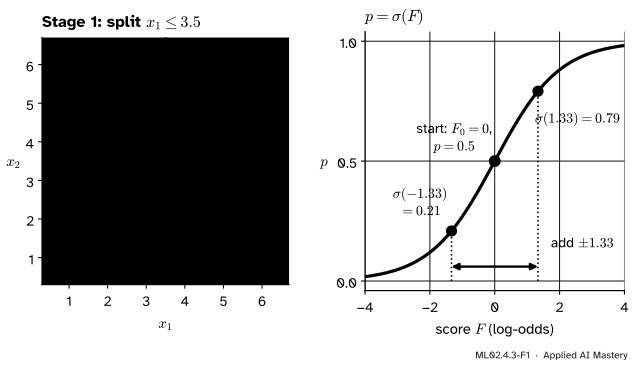
Take the twelve points of the course, six of class 0 and six of class 1. Half are in class 1, so the starting probability is \(0.5\) and the starting score is \(F_0 = 0\). The first stump splits at \(x_1 \le 3.5\), where five of six points are class 0 on the left and five of six are class 1 on the right, and it adds \(-1.33\) on the left and \(+1.33\) on the right.
ML02.4.3-F1
Left: the first stump adds \(-1.33\) to the score on one side and \(+1.33\) on the other. Right: the sigmoid turns the score into a probability, \(0.21\) and \(0.79\).
The trees work on the scale where adding is safe; only the final score is squeezed into \((0, 1)\). Two questions remain: what the trees are fitted to, and why the leaf value is \(1.33\).
Build it up
Step 1. The loss in terms of the score. For a label \(y \in \{0, 1\}\) and \({p = \sigma(F)}\), the log loss is \({L = -[\,y \ln p + (1 - y) \ln(1 - p)\,]}\). Written with \(F\) it becomes \({L(y, F) = \ln(1 + e^{F}) - yF}\), derived below.
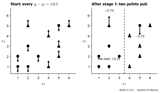
Step 2. The pseudo-residual is \(y - p\). The derivative of \(L\) with respect to \(F\) is \({p - y}\), so the negative gradient is \({y - p}\): the label minus the predicted probability. For a class-1 point predicted at \(0.21\), it is \(+0.79\), a strong pull upwards.
ML02.4.3-F2
The pseudo-residuals \({y_i - p_i}\) as arrows. At the start every point pulls equally. After one stage, the ten points on the right side of the split pull weakly and the two misplaced points pull hard; the next tree is fitted to these arrows.
Step 3. The leaf value has no formula. Step 2c of the algorithm asks for the \(\gamma\) that minimises \({\sum \ln(1 + e^{F_i + \gamma}) - y_i (F_i + \gamma)}\) over a leaf. Setting its derivative to zero gives \({\sum \sigma(F_i + \gamma) = \sum y_i}\), which cannot be solved for \(\gamma\) in closed form once the \(F_i\) differ.
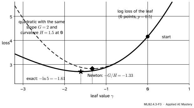
Step 4. One Newton step instead. Replace the leaf’s loss by its second-order Taylor polynomial at \(\gamma = 0\) (M04.8) and minimise that. It needs only the first and second derivatives of each point’s loss, which are \({p_i - y_i}\) and \({p_i(1 - p_i)}\).
The formal statement
The loss as a function of the score. From \({p = e^{F}/(1 + e^{F})}\),
\[
\begin{aligned}
\ln p &= F - \ln(1 + e^{F}), \\
\ln(1 - p) &= -\ln(1 + e^{F}).
\end{aligned}
\]
Its derivatives. The derivative of \({\ln(1 + e^{F})}\) is \({e^{F}/(1 + e^{F}) = p}\), so
\[
\begin{aligned}
g &= \pd{L}{F} = p - y, \\
h &= \frac{\partial^2 L}{\partial F^2} = p(1 - p),
\end{aligned}
\]
where the second uses \({\sigma'(F) = \sigma(F)(1 - \sigma(F))}\) from ML01.6. The curvature \(h\) is largest, \(\tfrac14\), at \(p = 0.5\) and tiny when the model is confident.
The starting score. The best constant \(c\) makes \({\sum_i (\sigma(c) - y_i)}\) zero, so \({\sigma(c) = \bar{y}}\), the fraction of class 1. Solving for \(c\),
\[
F_0 = \ln \frac{\bar{y}}{1 - \bar{y}},
\]
the log-odds of the base rate.
NoteResult: the Newton leaf value
For the points of one leaf, with current probabilities \(p_i\), write the leaf sums \({G = \sum (p_i - y_i)}\) and \({H = \sum p_i (1 - p_i)}\). The second-order Taylor expansion of the leaf’s loss in \(\gamma\) is
The numerator is the sum of the pseudo-residuals, the denominator the sum of the curvatures. Where the model is unsure (\(p\) near \(0.5\)) the curvature is large and the step is modest; where it is confident the same residual buys a bigger step.
ML02.4.3-F3
The Newton step for the left leaf of stage 1. The dashed quadratic matches the loss in value, slope and curvature at \(\gamma = 0\); its minimum, \(-1.33\), lands close to the true minimum, \(-1.61\).
Go deeper: many classes: K trees per stage
With \(K\) classes the model keeps \(K\) scores \(F_k\), turned into probabilities by the softmax (ML02.10.1), and the log loss gives pseudo-residuals \({y_{ik} - p_{ik}}\) for each class, where \(y_{ik}\) is \(1\) for the true class and \(0\) otherwise (ESL equation 10.38). Each stage fits one tree per class. Using only the diagonal of the Hessian, the Newton leaf value for class \(k\) is \({\sum (y_{ik} - p_{ik}) / \sum p_{ik}(1 - p_{ik})}\) (ESL Exercise 10.8, equation 10.57). ESL then centres the \(K\) values so that they sum to zero and multiplies them by \({(K - 1)/K}\) (equation 10.58). For \(K = 2\) one tree per stage is enough (ESL Exercise 10.10), which is the binary case of this lesson.
Frontier note: the seed of XGBoost
The Newton value \({-G/H}\) is where XGBoost begins. Lesson ML02.5.1 adds a penalty \(\tfrac12 \lambda \gamma^2\) to each leaf, which turns the value into \({-G/(H + \lambda)}\), and uses the same quadratic to score every candidate split, not only to set the leaves.
Worked example
Labels: class 0 is \(y = 0\) at \((1, 1)\), \((2, 1)\), \((1, 2)\), \((2, 3)\), \((3, 2)\), \((5, 5)\) and class 1 is \(y = 1\) at \((4, 1)\), \((5, 2)\), \((5, 3)\), \((4, 4)\), \((2, 5)\), \((6, 5)\). Learning rate \(\cparam{\nu} = 1\), stumps.
Start.\({\bar{y} = 0.5}\), so \({F_0 = \ln 1 = 0}\) and every \({p_i = 0.5}\). The pseudo-residuals are \(\pm 0.5\) and the log loss is \({\ln 2 \approx 0.693}\).
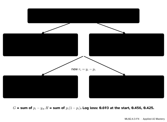
Stage 1. A stump fitted to the \(\pm 0.5\) by squared error splits at \(x_1 \le 3.5\). The left leaf has five class-0 points and one class-1 point:
The right leaf is the mirror image, \({\gamma = +4/3}\). So \({F_1 = \pm 1.33}\) and \({p = \sigma(\pm 4/3)}\), which is \(0.79\) or \(0.21\). Ten points are now on the right side; \((2, 5)\) and \((5, 5)\) are not. The log loss falls to \(0.456\).
Stage 2. Write \({q = \sigma(4/3) \approx 0.7914}\). The pseudo-residuals are \({\pm(1 - q) = \pm 0.209}\) for the ten well-placed points and \({\pm q = \pm 0.791}\) for the two misplaced ones. The best stump by squared error splits at \(x_1 \le 1.5\), isolating \((1, 1)\) and \((1, 2)\) (squared error \(1.583\), against \(1.622\) for the runner-up \(x_2 \le 3.5\)). Both points are class 0 with \({p = 1 - q}\):
The other ten points have \({G \approx -0.417}\) (the total of all \(p_i - y_i\) is still zero) and \({H = 10\,q(1 - q) \approx 1.651}\), so \({\gamma = 1/(5q) \approx 0.253}\). The scores become \(-2.60\) for \((1, 1)\) and \((1, 2)\), \(-1.08\) for the other points with \(x_1 \le 3.5\) and \(+1.59\) for the rest, and the log loss falls to \(0.425\).
ML02.4.3-F4
Two stages, leaf by leaf. Each leaf value is \({-G/H}\), computed from the probabilities of the points that land in it.
A stump can only cut along one axis, so the two misplaced points \((2, 5)\) and \((5, 5)\) stay on the wrong side: the training accuracy is \(10/12\) after both stages. Deeper trees, or more stages, can isolate them.
Code
From scratch: the stump finder of lesson ML02.4.1, run over both features, with the Newton leaf.
import numpy as npX = np.array([(1, 1), (2, 1), (1, 2), (2, 3), (3, 2), (5, 5), (4, 1), (5, 2), (5, 3), (4, 4), (2, 5), (6, 5)], dtype=float)y = np.array([0] *6+ [1] *6, dtype=float)sigmoid =lambda z: 1/ (1+ np.exp(-z))def best_split(X, r): best =Nonefor j inrange(X.shape[1]): values = np.unique(X[:, j])for s in (values[:-1] + values[1:]) /2: left = X[:, j] <= s sse = ((r[left] - r[left].mean()) **2).sum() + ((r[~left] - r[~left].mean()) **2).sum()if best isNoneor sse < best[2] -1e-12: best = (j, s, sse)return best[:2]def newton(y, p):return (y - p).sum() / (p * (1- p)).sum()def boost_classifier(X, y, stages, nu=1.0): F = np.full(len(y), np.log(y.mean() / (1- y.mean()))) trees, scores = [], []for _ inrange(stages): p = sigmoid(F) j, s = best_split(X, y - p) # tree fitted to the pseudo-residuals y - p left = X[:, j] <= s a, b = newton(y[left], p[left]), newton(y[~left], p[~left]) trees.append((j, s, a, b)) F = F + nu * np.where(left, a, b) scores.append(F.copy())return trees, scoreslog_loss =lambda F: -np.mean(y * np.log(sigmoid(F)) + (1- y) * np.log(1- sigmoid(F)))trees, scores = boost_classifier(X, y, stages=2)for (j, s, a, b), F inzip(trees, scores):print(f"x{j +1} <= {s}: leaves {a:+.3f}{b:+.3f} log loss {log_loss(F):.3f}")
x1 <= 3.5: leaves -1.333 +1.333   log loss 0.456
x1 <= 1.5: leaves -1.264 +0.253   log loss 0.425
Now GradientBoostingClassifier. Its trees are regression trees, it starts from the log-odds of the base rate, and its leaf values are this same Newton step; staged_decision_function returns the score \(F_m\) after each stage.
from sklearn.ensemble import GradientBoostingClassifiergbc = GradientBoostingClassifier(n_estimators=2, learning_rate=1.0, max_depth=1).fit(X, y)library = [F.ravel() for F in gbc.staged_decision_function(X)]print("same scores:", all(np.allclose(a, b) for a, b inzip(library, scores)))print("p for (2, 5) and (5, 5):", np.round(gbc.predict_proba(X[[10, 5]])[:, 1], 3))
same scores: True
p for (2, 5) and (5, 5): [0.253 0.83 ]
Explore
The module’s interactive, the residual stepper, is in lesson ML02.4.1. It boosts a regression target; the classifier of this lesson runs the same loop with \({y - p}\) in place of \({y - F}\) and the Newton value in each leaf.
Pitfalls
ML02.4.3-F5
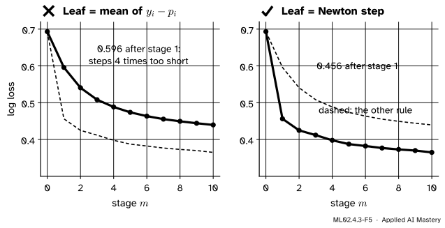
Wrong beside right. With the mean residual as the leaf value, the first step is \({-1/3}\) instead of \({-4/3}\): at \({p = 0.5}\) every curvature is \({\tfrac14}\), so the plain gradient step is four times too short, and it takes seven stages to get as low as one Newton stage.
“The leaf value is the average pseudo-residual, as in regression.”
That is the squared-loss rule. For the log loss the residuals \({y - p}\) live on the probability scale while the leaves add to the log-odds; dividing by the curvature \({\sum p_i(1 - p_i)}\) converts one to the other.
“The boosted score is a probability.”
\(F\) is a log-odds. After stage 1 the scores are \(\pm 1.33\), not probabilities; apply the sigmoid to get \(0.21\) and \(0.79\). In scikit-learn, decision_function returns \(F\) and predict_proba returns \(\sigma(F)\).
“Each tree is a classifier that votes, as in AdaBoost.”
In gradient boosting every tree is a regression tree fitted to real-valued pseudo-residuals, and its leaves hold real numbers that add up. scikit-learn’s guide says it plainly: even for classification, the sub-estimator is a regressor.
Check yourself
Recall
1. Write the log loss as a function of the score \(F\), for a label \({y \in \{0, 1\}}\).
Show answer
\({L(y, F) = \ln(1 + e^{F}) - yF}\).
2. What are the first and second derivatives of that loss with respect to \(F\)?
Show answer
\({p - y}\) and \({p(1 - p)}\), with \({p = \sigma(F)}\).
3. What is the starting score \(F_0\) when 30 percent of the training labels are 1?
Show answer
The log-odds of the base rate: \({\ln(0.3/0.7) \approx -0.847}\).
4. Give the Newton leaf value in terms of the leaf sums \(G\) and \(H\).
Show answer
\({\gamma = -G/H}\), with \({G = \sum (p_i - y_i)}\) and \({H = \sum p_i(1 - p_i)}\) over the points in the leaf.
5. On the twelve points with \({\cparam{\nu} = 1}\), what are the stage-1 leaf values and probabilities?
Show answer
\({\mp 4/3}\) on either side of \(x_1 = 3.5\), giving probabilities \(0.21\) on the left and \(0.79\) on the right.
Exercises
1.★ A leaf holds four points with labels (1, 1, 1, 0), all with current probability \({p = 0.8}\). Compute \(G\), \(H\) and the Newton leaf value, and the new probability.
Show solution
\(G = {3(0.8 - 1)} + {(0.8 - 0)} = 0.2\) and \(H = {4 \times 0.8 \times 0.2} = 0.64\), so \({\gamma = -0.2/0.64 = -0.3125}\). The score was \({\ln(0.8/0.2) = \ln 4 \approx 1.386}\); it becomes about \(1.074\), and \({\sigma(1.074) \approx 0.745}\), close to the leaf’s base rate \(0.75\).
2.★★ Show that for a leaf whose points all share the same current probability \(p\), with \(k\) points of which \(k_1\) are class 1, the Newton value is \({(\bar{y}_\ell - p) / (p(1 - p))}\), where \({\bar{y}_\ell = k_1/k}\). Compare it with the exact minimiser \({\ln \frac{\bar{y}_\ell}{1 - \bar{y}_\ell} - \ln \frac{p}{1 - p}}\) for the left leaf of stage 1.
Show solution
\({\sum (y_i - p) = k_1 - kp = k(\bar{y}_\ell - p)}\) and \({\sum p(1 - p) = k\,p(1 - p)}\); the \(k\) cancels. When all scores in the leaf are equal, the exact minimiser moves them to the score whose probability is the leaf’s base rate, \({\sigma(F + \gamma) = \bar{y}_\ell}\), which gives the difference of log-odds. For the left leaf, \({\bar{y}_\ell = 1/6}\) and \({p = 1/2}\): Newton gives \({(1/6 - 1/2)/(1/4) = -4/3}\), and the exact value is \({\ln(1/5) - 0 = -\ln 5 \approx -1.609}\).
3.★★★ Show that the Newton step is exact for the squared loss \({\tfrac12(y - F)^2}\), and explain why the classification step 2c needs an approximation while regression does not.
Show solution
For the squared loss, \({g_i = F_i - y_i}\) and \({h_i = 1}\), so \({-G/H = \frac1k \sum (y_i - F_i)}\), the mean residual, which is the exact minimiser of Fact 1 of lesson ML02.4.1. The Taylor expansion of a quadratic to second order is the quadratic itself, so nothing is lost. The log loss \({\ln(1 + e^{F}) - yF}\) has derivatives of every order, so its second-order polynomial is only an approximation, and the exact minimiser solves \({\sum \sigma(F_i + \gamma) = \sum y_i}\), which has no closed form when the \(F_i\) differ.
Summary card
Boost the log-odds; fit trees to \({y - p}\); set each leaf by one Newton step.
Leaf.\({\gamma = -G/H}\), with \({G = \sum (p_i - y_i)}\) and \({H = \sum p_i(1 - p_i)}\).
Twelve points. Log loss \({0.693 \to 0.456 \to 0.425}\).
Sources and next steps
Sources. Each was opened and checked against this lesson on 15 November 2026.
Trevor Hastie, Robert Tibshirani and Jerome Friedman, The Elements of Statistical Learning, 2nd edition, 12th printing. Table 10.2 gives the negative gradient of the deviance as \({I(y_i = G_k) - p_k(x_i)}\), equation 10.38 builds one tree per class, and Algorithm 10.3 is repeated \(K\) times per iteration. Exercise 10.8 derives the one-step approximate Newton update \({\sum (y_{ik} - p_{ik}) / \sum p_{ik}(1 - p_{ik})}\) (equation 10.57) and its \({(K - 1)/K}\) rescaling (10.58); Exercise 10.10 shows one tree suffices for two classes.
scikit-learn developers, User Guide 1.11.1.2.3, version 1.9.1. For the log loss, the probability of the positive class is the sigmoid of \(F_M(x_i)\), the initial model is the log odds-ratio, and “even for a classification task, the \(h_m\) sub-estimator is still a regressor”. The Newton leaf value \({\sum (y - p) / \sum p(1 - p)}\) was read in the library’s source, _update_terminal_regions in sklearn/ensemble/_gb.py.