\( \newcommand{\vect}[1]{\boldsymbol{\mathbf{#1}}} \newcommand{\mat}[1]{\boldsymbol{\mathbf{#1}}} \newcommand{\R}{\mathbb{R}} \newcommand{\E}{\mathbb{E}} \newcommand{\Prob}{\mathbb{P}} \newcommand{\T}{^{\top}} \newcommand{\norm}[1]{\lVert #1 \rVert} \newcommand{\abs}[1]{\lvert #1 \rvert} \newcommand{\ihat}{\mkern1mu\hat{\boldsymbol{\imath}}\mkern2mu} \newcommand{\jhat}{\mkern1mu\hat{\boldsymbol{\jmath}}\mkern2mu} \newcommand{\pd}[2]{\frac{\partial #1}{\partial #2}} \newcommand{\argmax}{\operatorname*{arg\,max}} \newcommand{\argmin}{\operatorname*{arg\,min}} \newcommand{\cdata}[1]{\class{c-data}{#1}} \newcommand{\cmodel}[1]{\class{c-model}{#1}} \newcommand{\ctruth}[1]{\class{c-truth}{#1}} \newcommand{\cgrad}[1]{\class{c-grad}{#1}} \newcommand{\closs}[1]{\class{c-loss}{#1}} \newcommand{\cparam}[1]{\class{c-param}{#1}} \newcommand{\csecond}[1]{\class{c-second}{#1}} \renewcommand{\,}{\mkern3mu} \)

Every model makes an assumption

A tree assumes boxes, a linear model one straight cut, k-nearest neighbours that near points agree, naive Bayes one feature at a time. Fit all four to the same four datasets and see each assumption help on one and hurt on another.

ML02.11.1L2 Intermediate25 min

In review

The maths and code on this page are checked by automated tests on every change, but an independent reader has not signed it off yet. Spot a mistake or a confusing step? Tell us.

Before this lesson: ML01.3 k-nearest neighbors ML01.6 Logistic regression and classification ML02.1 Decision trees ML02.6 Naive Bayes and generative classifiers

What you will be able to do

Name the inductive bias of trees, linear models, k-nearest neighbours and naive Bayes, and sketch the boundary shape each one draws easily.
Predict which family will struggle on a diagonal boundary, on rings and on data with irrelevant features, and check the prediction by fitting.
Show that an irrelevant standardised feature adds 2 on average to a squared distance, and explain what that does to k-nearest neighbours.
State the no-free-lunch idea in words and explain why it does not make all models equal on real data.

The question

You have met a tree, a straight-line classifier, \(k\)-nearest neighbours and naive Bayes. Fit all four to the same small dataset and one of them wins clearly. Fit them to a second dataset and a different one wins, and the first winner may score no better than a coin. Which model is best? And can you tell before you fit anything?

Intuition

Two hundred points cannot pin down a boundary. Infinitely many boundaries pass between them, and each model picks one by a rule built in before it sees any data. That built-in preference is the model’s inductive bias: the shapes it can draw cheaply, and the ones it can only imitate.

A tree cuts the plane with lines parallel to the axes. Logistic regression draws one straight line. Each shape is right exactly when the data are shaped that way.

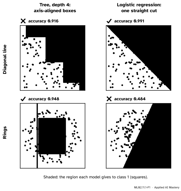
ML02.11.1-F1

The same two models on two datasets. On the diagonal line, logistic regression’s straight cut is exactly the right shape and the tree can only climb a staircase. On the rings, the tree boxes in the middle and the straight line is useless. Each model wins where its assumption matches.

The accuracies are measured on 1,000 fresh points from the same source, not on the 200 the model saw. Look at the bottom right: 0.484 is no better than guessing. Logistic regression did not fail to train. It found the best straight line, and the best straight line is useless here.

Build it up

Four families appear in this course, and each has one assumption at its heart.

Step 1. Trees assume boxes. A tree asks one question about one feature at a time (ML02.1.1), so its regions are rectangles with sides parallel to the axes. Forests and boosted trees (ML02.2 to ML02.5) add many trees together, but each piece is still a box. Their boundaries are made of axis-parallel steps.

Step 2. Linear models assume one straight cut. Logistic regression (ML01.6), linear discriminant analysis and the linear SVM (ML02.7) all compute a score \(\vect{w}\cdot\vect{x} + b\) and compare it with a threshold. The boundary is a straight line in the plane, a flat plane or hyperplane in more dimensions.

Step 3. \(k\)-nearest neighbours assume that near points agree (ML01.3). So does an SVM with an RBF kernel (ML02.8), whose kernel is large only for nearby points. Their boundaries bend to follow the data, but “near” is measured with every feature, whether it matters or not.

Step 4. Naive Bayes assumes the features are independent within each class (ML02.6). Its evidence for a class is a sum of one term per feature, so it cannot see a pattern that lives in two features together.

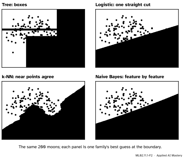
ML02.11.1-F2

Four assumptions, four shapes, on the moons. Only \(k\)-nearest neighbours can follow the curl of the moons, because only it is free to bend wherever the points do.

Step 5. The full line-up. Fit the four families to four datasets: the diagonal line, the moons, the rings, and two overlapping round clouds (“blobs”) with a third feature of pure noise.

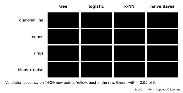
ML02.11.1-F6

The scoreboard. Yellow marks the best in each row and green anything within \(0.02\) of it. The winner changes from row to row, and the logistic column runs from first place to last.

Read the rows one at a time. The diagonal line suits linear models. The moons suit a model that bends. On the rings the straight line collapses, but naive Bayes scores \(0.979\): a surprise that the formal section explains. On the blobs the true boundary is a straight line and the classes overlap. Logistic regression and naive Bayes land near the best possible accuracy, about \(0.87\); the noise feature costs \(k\)-NN a little, and the tree trails.

The depth-4 tree wins no row. Alone, it is rarely the best model. Its strengths (Lesson 2) are elsewhere, and its ensembles are much stronger.

The formal statement

Definition: inductive bias

The inductive bias of a learning method is everything other than the data that decides which function it returns: the set of functions it can represent, and its preferences among those that fit the data equally well.

Here are the four families written so that their biases can be read off.

Trees. With leaves that cover regions \(R_1, \dots, R_M\) of the feature space, a tree predicts

\[ \cmodel{f(\vect{x})} = \sum_{m=1}^{M} c_m \, I(\vect{x} \in R_m), \]

where \(I(\cdot)\) is 1 when the condition holds and 0 otherwise, and each \(R_m\) is a box with sides parallel to the axes. A diagonal boundary needs many small boxes.

Linear models. Predict class 1 when \(\vect{w}\cdot\vect{x} + b \ge 0\). The boundary is the set where the score is exactly zero, a hyperplane.

\(k\)-nearest neighbours. The squared distance adds one term per feature:

\[ \norm{\vect{x} - \vect{z}}^2 = \sum_{j=1}^{d} (x_j - z_j)^2 . \]

Every feature counts equally, whether or not it has anything to do with the label.

Result 1: an irrelevant feature adds 2, on average. Let feature \(j\) be pure noise, standardised to mean \(\mu = 0\) and variance \(\sigma^2 = 1\), and let \(x_j\) and \(z_j\) be its values for two independent examples. Expand the square and take expectations term by term:

\[ \begin{aligned} &\E[(x_j - z_j)^2] \\ &\quad= \E[x_j^2] + \E[z_j^2] - 2\,\E[x_j z_j] \\ &\quad= \E[x_j^2] + \E[z_j^2] - 2\mu^2 \\ &\quad= 2(\sigma^2 + \mu^2) - 2\mu^2 \\ &\quad= 2\sigma^2 = 2 . \end{aligned} \]

Independence gives \({\E[x_j z_j]} = {\E[x_j]\,\E[z_j]} = \mu^2\) in the third line, and \(\E[x^2] = {\sigma^2 + \mu^2}\) gives the fourth. The noise adds the same amount whatever the classes of the two examples. Near neighbours in the real features differ by much less than 2, so a few noise features can drown them.

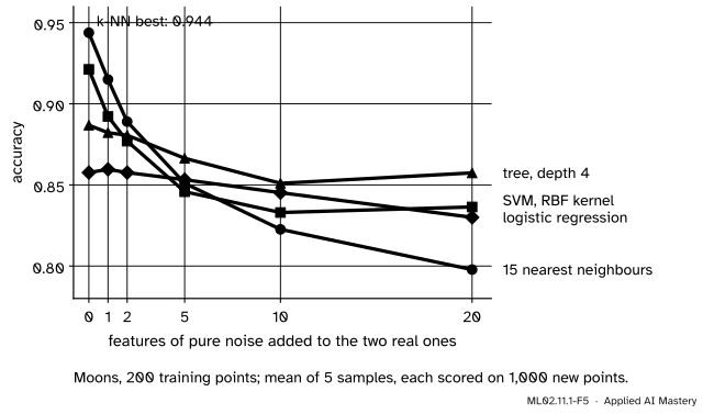
ML02.11.1-F5

Noise features added to the moons. The two distance-based models start best and fall furthest. The tree, which picks one feature per question, barely notices.

Naive Bayes. By Bayes’ rule and the naive assumption (ML02.6.2), the log-odds of class 1 is a sum of one term per feature:

\[ \begin{aligned} &\ln \frac{\Prob(y = 1 \mid \vect{x})}{\Prob(y = 0 \mid \vect{x})} \\ &\quad= \ln\frac{\pi_1}{\pi_0} + \sum_{j=1}^{d} \ln \frac{p(x_j \mid 1)}{p(x_j \mid 0)} . \end{aligned} \]

Result 2: Gaussian naive Bayes draws circles but not crosses. With one Gaussian per feature per class, each term is

\[ \begin{aligned} \ln \frac{p(x_j \mid 1)}{p(x_j \mid 0)} &= \ln\frac{\sigma_{0j}}{\sigma_{1j}} - \frac{(x_j - \mu_{1j})^2}{2\sigma_{1j}^2} \\ &\quad + \frac{(x_j - \mu_{0j})^2}{2\sigma_{0j}^2}, \end{aligned} \]

a quadratic in \(x_j\) alone. So the boundary has the form \({a_1 x_1^2 + b_1 x_1} + {a_2 x_2^2 + b_2 x_2} + c = 0\). When \(a_1 = a_2\) that is a circle, which is why naive Bayes handles the rings: the inner ring has the smaller spread in each feature. No product \(x_1 x_2\) can appear, so a pattern like “class 1 when both features have the same sign” is out of reach.

The no-free-lunch idea. No learning method is best on every problem. For any method there is a problem on which it fails while another method succeeds. A good fit always comes from an assumption that matches the data, never from the method alone.

Go deeper: the theorem behind the slogan

Shalev-Shwartz and Ben-David (Theorem 5.1) make this precise for classification. Take any learning algorithm and any training-set size \(m\) smaller than half the number of possible inputs. Then some distribution of labelled data exists for which a perfect classifier exists, yet with probability at least \(1/7\) the algorithm’s error is at least \(1/8\). The proof hides the labels of the unseen half of the inputs: an algorithm that has seen half the points knows nothing about the rest unless it assumes something. Their Section 5.1.1 draws the moral: prior knowledge, expressed as a restricted set of functions, is what makes learning possible.

Worked example

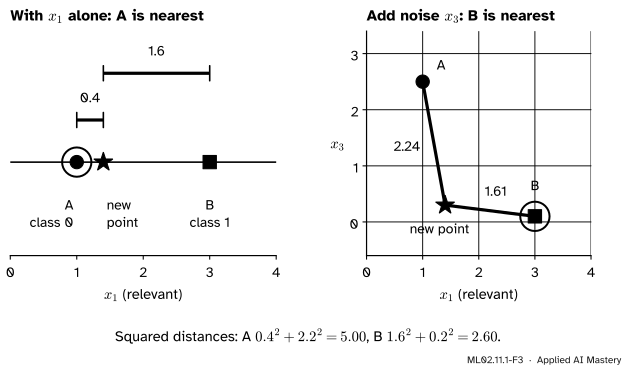
One noise feature misleads \(k\)-NN. Two training points and a new point, with one relevant feature \(x_1\) and one feature of noise \(x_3\):

Point	\(x_1\)	\(x_3\)	class
A	\(1.0\)	\(2.5\)	0
B	\(3.0\)	\(0.1\)	1
new	\(1.4\)	\(0.3\)	?

ML02.11.1-F3

The same three points with and without the noise feature. The noise in \(x_3\) outweighs the real difference in \(x_1\).

With \(x_1\) alone. The distance to A is \({\abs{1.4 - 1.0}} = 0.4\) and to B is \({\abs{1.4 - 3.0}} = 1.6\). The nearest neighbour is A, so 1-NN predicts class 0.

With \(x_3\) added. The squared distance to A is

\[ \begin{aligned} &(1.4 - 1.0)^2 + (0.3 - 2.5)^2 \\ &\quad= 0.16 + 4.84 = 5.00, \end{aligned} \]

so the distance is \(\sqrt{5.00} = 2.24\). To B it is

\[ \begin{aligned} &(1.4 - 3.0)^2 + (0.3 - 0.1)^2 \\ &\quad= 2.56 + 0.04 = 2.60, \end{aligned} \]

so the distance is \(\sqrt{2.60} = 1.61\). Now B is nearer and 1-NN predicts class 1.

The noise feature contributed \(4.84\) of A’s \(5.00\). By Result 1 it adds 2 on average when standardised, so this draw was unlucky, but with ten noise features the expected extra is 20, and nothing in the distance tells signal from noise. A tree would ask about \(x_1\) and never look at \(x_3\).

Code

The four datasets and the four models, exactly as in the figures.

import numpy as np
from sklearn.datasets import make_circles, make_moons
from sklearn.linear_model import LogisticRegression
from sklearn.naive_bayes import GaussianNB
from sklearn.neighbors import KNeighborsClassifier
from sklearn.pipeline import make_pipeline
from sklearn.preprocessing import StandardScaler
from sklearn.tree import DecisionTreeClassifier

def line(n, seed):
    rng = np.random.default_rng(seed)
    X = rng.uniform(-3, 3, size=(n, 2))
    return X, (X[:, 0] + X[:, 1] > 0).astype(int)              # class 1 above the diagonal

def blobs(n, seed, extra=1):
    rng = np.random.default_rng(seed)
    y = rng.integers(0, 2, n)
    s = np.where(y == 1, 1.0, -1.0)                             # means (-1, -0.5) and (1, 0.5)
    X = np.column_stack([rng.normal(s, 1.0), rng.normal(0.5 * s, 1.0), rng.normal(0, 1, (n, extra))])
    return X, y

sets = {"line": line,
        "moons": lambda n, seed: make_moons(n, noise=0.25, random_state=seed),
        "rings": lambda n, seed: make_circles(n, noise=0.1, factor=0.5, random_state=seed),
        "blobs": blobs}
models = {"tree": lambda: DecisionTreeClassifier(max_depth=4, random_state=0),
          "logistic": lambda: make_pipeline(StandardScaler(), LogisticRegression()),
          "knn": lambda: make_pipeline(StandardScaler(), KNeighborsClassifier(15)),
          "naive Bayes": lambda: GaussianNB()}

board = {}
for name, make_set in sets.items():
    X_train, y_train = make_set(200, 0)                         # 200 to learn from
    X_val, y_val = make_set(1000, 1)                            # 1,000 fresh points to score on
    board[name] = {m: make().fit(X_train, y_train).score(X_val, y_val) for m, make in models.items()}
    print(f"{name:6}", "  ".join(f"{m} {s:.3f}" for m, s in board[name].items()))

line   tree 0.916  logistic 0.991  knn 0.965  naive Bayes 0.976
moons  tree 0.855  logistic 0.863  knn 0.930  naive Bayes 0.855
rings  tree 0.948  logistic 0.484  knn 0.990  naive Bayes 0.979
blobs  tree 0.832  logistic 0.860  knn 0.852  naive Bayes 0.855

From scratch, Result 1 and the worked example. Pairs of standardised noise values differ by 2 in square, on average, and one noise feature flips the nearest neighbour.

rng = np.random.default_rng(0)
u, v = rng.normal(size=(2, 100_000))
print(f"mean of (u - v)^2 over 100,000 pairs: {np.mean((u - v) ** 2):.3f}")

A, B, new = np.array([1.0, 2.5]), np.array([3.0, 0.1]), np.array([1.4, 0.3])
for cols, label in [([0], "x1 only"), ([0, 1], "x1 and x3")]:
    dA, dB = np.linalg.norm(new[cols] - A[cols]), np.linalg.norm(new[cols] - B[cols])
    print(f"{label:10} distance to A {dA:.2f}, to B {dB:.2f}: nearest is {'A' if dA < dB else 'B'}")

mean of (u - v)^2 over 100,000 pairs: 2.001
x1 only    distance to A 0.40, to B 1.60: nearest is A
x1 and x3  distance to A 2.24, to B 1.61: nearest is B

Now Gaussian naive Bayes from scratch on the rings, written as the sum of one-feature terms of Result 2, and checked against GaussianNB.

X_train, y_train = sets["rings"](200, 0)
X_val, y_val = sets["rings"](1000, 1)
prior = np.array([np.mean(y_train == k) for k in (0, 1)])
mu = np.array([X_train[y_train == k].mean(axis=0) for k in (0, 1)])
var = np.array([X_train[y_train == k].var(axis=0) for k in (0, 1)])     # maximum likelihood: divide by n

def term(x, k):                                                  # ln p(x_j | k), one column per feature
    return -0.5 * np.log(2 * np.pi * var[k]) - (x - mu[k]) ** 2 / (2 * var[k])

log_odds = np.log(prior[1] / prior[0]) + (term(X_val, 1) - term(X_val, 0)).sum(axis=1)
mine = (log_odds > 0).astype(int)
library = GaussianNB().fit(X_train, y_train).predict(X_val)
print("spread of each feature, outer ring (class 0):", np.sqrt(var[0]).round(2), " inner ring:", np.sqrt(var[1]).round(2))
print(f"accuracy {np.mean(mine == y_val):.3f}; agrees with GaussianNB on {np.mean(mine == library):.1%} of points")

spread of each feature, outer ring (class 0): [0.71 0.7 ]  inner ring: [0.35 0.38]
accuracy 0.979; agrees with GaussianNB on 100.0% of points

The inner ring’s spread is about half the outer ring’s in both features, so the quadratic terms have the same sign and the boundary closes into a loop.

Last, the noise experiment of the figure, for \(k\)-NN and the tree: five samples of the moons with no noise features and with twenty.

def moons_noise(n, seed, extra):
    X, y = make_moons(n, noise=0.25, random_state=seed)
    return np.column_stack([X, np.random.default_rng(seed).normal(0, 1, (n, extra))]), y

for name in ("knn", "tree"):
    for extra in (0, 20):
        acc = [models[name]().fit(*moons_noise(200, 10 + s, extra)).score(*moons_noise(1000, 100 + s, extra))
               for s in range(5)]
        print(f"{name:4} with {extra:2} noise features: mean accuracy {np.mean(acc):.3f}")

knn  with  0 noise features: mean accuracy 0.944
knn  with 20 noise features: mean accuracy 0.798
tree with  0 noise features: mean accuracy 0.887
tree with 20 noise features: mean accuracy 0.857

\(k\)-NN drops from \(0.944\) to \(0.798\); the tree from \(0.887\) to \(0.857\).

Explore

ML02.11-X1

Model line-up

Pick a dataset and watch four models draw their boundaries side by side, each with its accuracy on fresh points. Slide the training-set size down to 20 and up to 400.

Four panels of the same moons points with the boundaries of a tree (axis-aligned steps), logistic regression (one straight line), k-nearest neighbours (a wiggly curve following the moons) and Gaussian naive Bayes (a gently curved line), each with its validation accuracy.

Things to try.

Diagonal line, smallest training set. Logistic regression is already about 0.9; the tree needs many more points before its staircase hugs the line.
Rings. Logistic regression never gets far above one half, at any size. More data cannot fix a wrong shape.
Blobs + noise feature. No model passes about \(0.87\), the best possible here. Turn the noise feature off and on, with a few new samples: one noise feature costs little, and the figure in the formal section shows what twenty cost.

Pitfalls

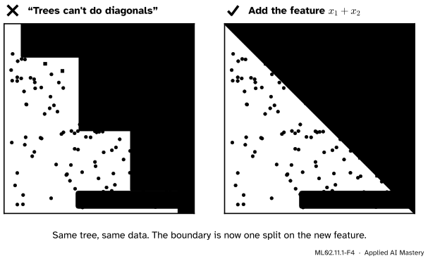
ML02.11.1-F4

Wrong beside right. The tree did not fail because trees are weak. It failed because its question does not match the shape. Give it the feature \(x_1 + x_2\) and one question is enough.

“Trees can’t learn diagonal boundaries, so trees are a poor choice here.”

A tree imitates a diagonal with a staircase and needs many points to make the steps fine. But the bias is about the features, not only the model. Add the feature \(x_1 + x_2\) and the same tree splits once, at \(x_1 + x_2 \approx 0\), with accuracy \(0.999\). Grinsztajn and colleagues make the matching point for tabular data: trees depend on the orientation of the features, and on real tables that is often a strength, because the columns mean something.

“The most flexible model is the safest choice.”

Flexibility costs data. \(k\)-NN can bend to any shape, yet with twenty noise features it fell to \(0.798\), below a depth-4 tree. A flexible model is safe only when the data are plentiful and the features are all relevant.

“No free lunch means every model is equally good, so the choice does not matter.”

The theorem’s argument ranges over every possible labelling of the inputs, including ones with no structure at all. Real tables have structure: smooth trends, a few strong features, meaningful columns. On real data some models are much better than others. The theorem only says the winner depends on the problem.

Check yourself

Recall

1. What is a model’s inductive bias?

Show answer

Everything other than the data that decides which function it returns: the functions it can represent and its preference among those that fit equally well.

2. What shape of boundary does each family draw easily: trees, linear models, \(k\)-NN?

Show answer

Trees: axis-parallel steps (boxes). Linear models: one straight line or hyperplane. \(k\)-NN: any curve that follows the local majority, with “near” measured on every feature.

3. Why did logistic regression score \(0.484\) on the rings?

Show answer

The boundary between the rings is a circle. The best straight line cannot separate an inner ring from an outer one, so it does no better than guessing.

4. On average, how much does one standardised noise feature add to a squared distance?

Show answer

\(2\), since \({\E[(x - z)^2]} = 2\sigma^2\) for two independent values with variance \(\sigma^2 = 1\).

5. State the no-free-lunch idea in one sentence.

Show answer

No learning method is best on every problem: for every method there is a problem on which another method does better.

Exercises

1. ★ A new point is at \(x_1 = 2.0\), \(x_3 = 1.0\). Training point C (class 0) is at \((2.5, 3.0)\) and D (class 1) at \((3.5, 1.2)\), written as \((x_1, x_3)\). Find the 1-NN prediction using \(x_1\) only, and using both features.

Show solution

With \(x_1\) only: distances \({\abs{2.0 - 2.5}} = 0.5\) to C and \({\abs{2.0 - 3.5}} = 1.5\) to D, so C is nearest and the prediction is class 0.

With both: to C, \({0.5^2 + 2.0^2} = {0.25 + 4} = 4.25\); to D, \({1.5^2 + 0.2^2} = {2.25 + 0.04} = 2.29\). D is nearest, so the prediction flips to class 1.

2. ★★ Which family would you expect to struggle on each of these, and why? (a) The label is 1 when \({x_1 > 0}\) and \({x_2 > 0}\) (a quadrant). (b) The label is 1 when \(x_1 x_2 > 0\) (same signs). (c) The label is 1 when \({x_2 > 0.3\,x_1}\).

Show solution

(a) Linear models: the corner of a quadrant is not a straight line. A tree needs just two splits.

(b) Linear models again, and naive Bayes: its log-odds is a sum of one-feature terms and cannot contain the product \(x_1 x_2\). If the points are spread evenly, each feature alone carries no information, since half of each class has \(x_1 > 0\). A tree can represent the pattern with three splits, though greedy growing may not find the first one (ML02.1.3). \(k\)-NN handles it easily.

3. ★★★ Show that if \(x_j\) and \(z_j\) are independent with means \(\mu_x \ne \mu_z\) and the same variance \(\sigma^2\), then \({\E[(x_j - z_j)^2]} = {2\sigma^2 + (\mu_x - \mu_z)^2}\). Use this to explain why a relevant feature helps \(k\)-NN and an irrelevant one hurts.

Show solution

Expand and use independence, \(\E[x_j z_j] = \mu_x \mu_z\):

\[ \begin{aligned} &\E[(x_j - z_j)^2] \\ &\quad= (\sigma^2 + \mu_x^2) - 2\mu_x\mu_z \\ &\qquad + (\sigma^2 + \mu_z^2) \\ &\quad= 2\sigma^2 + (\mu_x - \mu_z)^2 . \end{aligned} \]

Take \(x\) and \(z\) from different classes. A relevant feature has different class means, so it adds the extra \({(\mu_x - \mu_z)^2}\) to distances between classes and not to distances within a class: points of the other class look further away, which is what \(k\)-NN needs. An irrelevant feature has \(\mu_x = \mu_z\) and adds \(2\sigma^2\) to every distance alike, blurring the difference.

Summary card

Every model assumes a shape. It wins where the data have that shape.

The anchor figure again: a tree and logistic regression on a diagonal line and on rings. The straight line wins on the diagonal, 0.991 against 0.916, and the tree wins on the rings, 0.948 against 0.484. — ML02.11.1-F1
Each model wins one row.

Trees: \({f(\vect{x}) = \sum_m c_m I(\vect{x} \in R_m)}\), boxes with axis-parallel sides.
Linear: class 1 when \(\vect{w}\cdot\vect{x} + b \ge 0\), one hyperplane.
\(k\)-NN: every feature enters \(\norm{\vect{x} - \vect{z}}^2\); a noise feature adds 2 on average.
Naive Bayes: log-odds is a sum of one-feature terms; circles yes, products no.
No free lunch: no method is best on every problem.

Sources and next steps

Sources. Each was opened and checked against this lesson on 15 November 2026.

Gareth James, Daniela Witten, Trevor Hastie and Robert Tibshirani, An Introduction to Statistical Learning, 2nd edition (free PDF). Section 2.2: “There is no free lunch in statistics: no one method dominates all others over all possible data sets.” Section 8.1.3, equations 8.8 and 8.9 and Figure 8.7: a linear model beats a tree when the true boundary is linear, and a tree wins when it is made of axis-parallel pieces.
Shai Shalev-Shwartz and Shai Ben-David, Understanding Machine Learning: From Theory to Algorithms, Cambridge University Press, 2014 (free PDF). Theorem 5.1, the No-Free-Lunch theorem, with the constants \(1/7\) and \(1/8\), and Section 5.1.1 on prior knowledge.
Léo Grinsztajn, Edouard Oyallon and Gaël Varoquaux, Why do tree-based models still outperform deep learning on typical tabular data?, NeurIPS 2022 Datasets and Benchmarks Track. Section 5.3: uninformative features hurt some models more than trees. Section 5.4: data are not invariant to rotation, so a learning method need not be either.

Next. ML02.11.2 Matching the model to the data turns these biases into a checklist you can apply to a table before fitting anything.

This lesson unlocks

ML02.11.2 Matching the model to the data

Your progress is saved in this browser only. No account, no tracking.