A fully grown tree fits its training data perfectly and overfits. Prune it with minimal cost-complexity, derive the weakest-link sequence by hand, choose the price per leaf by cross-validation, and measure how much a single tree changes when the data are resampled.
ML02.1.4L2 Intermediate30 minIn review (what this means)
The maths and code on this page are checked by automated tests on every change, but an independent reader has not signed it off yet. Spot a mistake or a confusing step? Tell us.
Show with training and validation accuracy against depth that a fully grown tree overfits.
State the cost-complexity criterion R(T) + alpha |T| and derive the effective alpha at which a branch should be pruned.
Carry out weakest-link pruning by hand on a small tree and read the sequence of subtrees off a picture of lines.
Choose alpha by cross-validation with cost_complexity_pruning_path and ccp_alpha.
Measure the instability of a tree as the variance of its predictions over bootstrap resamples.
The question
Grown until every leaf is pure, a tree gets every training point right, however noisy the data. That cannot be a good sign. How large should a tree be, how do we cut a grown tree back to that size, and is one tree, even a well-pruned one, a reliable thing to trust?
From the last lesson
1. When does CART stop splitting a node?
Show answer
When the node is pure, when it reaches max_depth, when no split leaves at least min_samples_leaf points on each side, or when no split is possible at all.
2. Why can a greedy grower miss a small, perfect tree?
Show answer
It judges each split by its immediate impurity decrease. On a pattern like XOR every first split scores zero, so it cannot see that one of them enables a perfect tree one level down.
Intuition
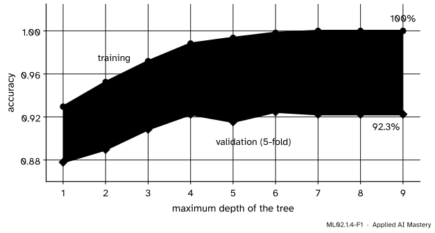
Take load_breast_cancer: 569 tumours, 30 measurements each, labelled malignant or benign. Split it as scikit-learn’s own pruning example does, 426 tumours to train and 143 to test. Grow trees of every depth on the training set and score them with 5-fold cross-validation (ML01.9).
ML02.1.4-F1
Training accuracy climbs to 100% as the tree deepens. Accuracy on held-out folds stops improving at about depth 4, so every split after that fits noise in the training set.
Each extra split makes the training fit better, never worse. The validation folds tell a different story: after about depth 4 the new splits buy nothing, because they chase the quirks of individual tumours. This is overfitting (ML01.8), and a tree is the clearest case of it: grown to the end, it can always reach 100% on the training set, unless two identical points disagree.
Build it up
Step 1. Grow big, then cut back. One fix is to stop early with max_depth. But the last lesson showed that a split that looks worthless may enable a good split below it. So the usual recipe grows a large tree first and then prunes it: it collapses some internal nodes into leaves.
Step 2. Put a price on leaves. Score a tree \(T\) by its training impurity plus a price \(\alpha \ge 0\) for every leaf:
\[
R_\alpha(T) = R(T) + \alpha\,|T| .
\]
Here \(|T|\) is the number of leaves and \(R(T)\) adds up the leaves’ impurities, each weighted by its share of the training points. With \(\alpha = 0\) the full tree wins, since it has \(R(T) = 0\). As \(\alpha\) grows, leaves become expensive and smaller trees win. This is the same idea as the penalty of ridge and lasso (ML01.9), with leaves in place of weights.
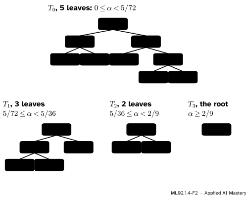
Step 3. Prune the weakest link first. As \(\alpha\) rises from 0, the best tree does not jump around: it loses one branch at a time, the one that buys the least impurity per leaf. That gives a short, nested list of trees, one for each range of \(\alpha\).
ML02.1.4-F2
Weakest-link pruning of the twelve-point tree. Each tree in the list is the previous one with one branch collapsed. Notice that the whole right side goes at once, before the left split.
Step 4. Choose \(\alpha\) by cross-validation. Each candidate \(\alpha\) gives one tree. Score each by cross-validation on the training set and keep the best, or, to allow for the noise in those scores, the simplest tree whose score is within one standard error of the best.
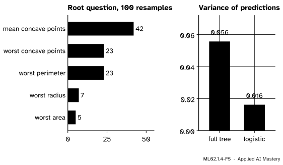
Step 5. Ask how stable the answer is. Draw a bootstrap sample of the training set: 426 draws with replacement, so that some tumours appear twice and others not at all. Grow a tree on it, and repeat 100 times. Each sample is a slightly different training set from the same source, the setting of the variance in ML01.8.2. The trees do not agree, not even on the first question.
ML02.1.4-F5
One hundred trees from one hundred bootstrap samples. Their first question uses five different features, and their predictions on the test tumours vary more than three times as much as those of logistic regression.
The formal statement
Let a tree be grown on \(n\) training points. For a node \(t\) holding \(n_t\) of them, with impurity \(I(t)\), write \(R(t) = \tfrac{n_t}{n} I(t)\). For a tree, \(R(T)\) is the sum of \(R\) over its leaves.
NoteDefinition: minimal cost-complexity pruning
For a price \(\cparam{\alpha} \ge 0\), the cost-complexity of a subtree \(T\) of the full tree is
\[
R_\alpha(T) = R(T) + \cparam{\alpha}\,|T| ,
\]
and \(T_\alpha\) is the smallest subtree with the least cost. scikit-learn uses the weighted Gini or entropy as \(R\); ISLR uses the squared error for regression, and ESL notes that the misclassification rate is the usual choice for classification. The method is the same.
When should one branch go? Take an internal node \(t\), and let \(T_t\) be the branch below it, with \(|T_t|\) leaves. Keeping the branch costs \(R(T_t) + \alpha|T_t|\). Collapsing it into the single leaf \(t\) costs \(R(t) + \alpha\). The two costs are equal when
Call this the effective alpha of \(t\), written \(\alpha_{\text{eff}}(t)\). It is the impurity the branch saves per extra leaf. For any larger \(\alpha\), collapsing is cheaper.
NoteAlgorithm: weakest-link pruning
Start with the full tree \(T_0\) and \(\alpha_0 = 0\).
Compute \(\alpha_{\text{eff}}(t)\) for every internal node of the current tree.
Collapse the node with the smallest one, the weakest link; record that value as the next \(\alpha_k\) and the pruned tree as \(T_k\).
Repeat from step 2 until only the root is left.
For \(\alpha_k \le \alpha < \alpha_{k+1}\) the tree \(T_k\) minimises \(R_\alpha\), so the whole path is found by one pass of collapses (Breiman, Friedman, Olshen and Stone, 1984; see ESL 9.2.2).
Go deeper: why no other subtree can win
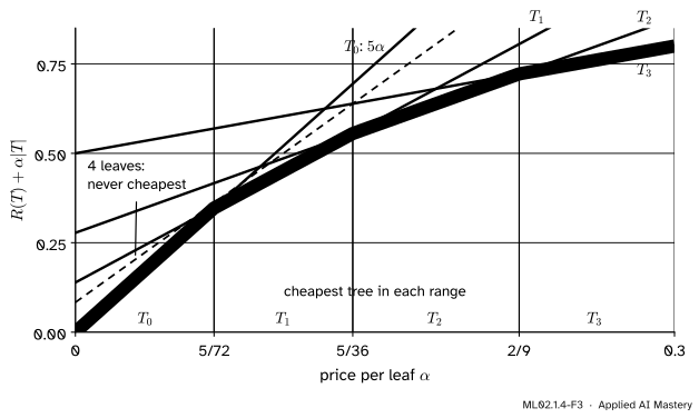
Every candidate subtree has cost \(R(T) + \alpha|T|\), a straight line in \(\alpha\) with slope \(|T|\). The cheapest tree at each \(\alpha\) is the lowest of these lines, their lower envelope. Moving right along the envelope, the slope can only fall, so the best tree only loses leaves as \(\alpha\) grows. At a corner of the envelope, the line of the current tree meets the line of a smaller one. Collapsing a single branch \(t\) moves you to the tree whose line meets the current one at \(\alpha_{\text{eff}}(t)\), and collapsing the branch with the smallest such value reaches the next corner first. Breiman and colleagues prove that the resulting trees are nested and that the smallest minimiser is unique for each \(\alpha\); the worked example shows a line that never touches the envelope.
Worked example
Prune the twelve-point tree. It has four internal nodes. With Gini impurity and \(n = 12\):
Round 1. The weakest link is the right node, at \(\alpha_1 = 5/72\). It is not the lowest split: the right branch spends two splits to save \(5/36\), only \(5/72\) per leaf, while the top-right split alone saves \(1/12\). Collapse the right node: \(T_1\) has 3 leaves and \(R(T_1) = 5/36\).
Round 2. Recompute. The left node still has \(5/36\). The root’s branch now has 3 leaves and \(R = 5/36\), so its value is \({(1/2 - 5/36)/2} = 13/72 \approx 0.181\). The weakest is the left node, at \(\alpha_2 = 5/36\). Collapse it: \(T_2\) is the stump, with \(R(T_2) = 5/18\).
Round 3. Only the root is left, at \({(1/2 - 5/18)/1} = 2/9\). So \(\alpha_3 = 2/9\), which is also the root split’s Gini decrease from lesson 2: with one split, the effective alpha is exactly the impurity it saves.
ML02.1.4-F3
Each subtree’s cost is a line in \(\alpha\); the cheapest tree is the lowest line (yellow). Its corners are the weakest-link values \(5/72\), \(5/36\) and \(2/9\). The tree that cuts only the bottom split (dashed) is never the cheapest, which is why the weakest-link path skips it.
Code
First the curve of the anchor figure: training and validation accuracy against depth.
depth 1     training 0.930  validation 0.878
depth 2     training 0.952  validation 0.890
depth 4     training 0.988  validation 0.923
depth 7     training 1.000  validation 0.923
depth None  training 1.000  validation 0.923
full tree: 16 leaves, depth 8  test accuracy 0.881
Next, weakest-link pruning from scratch. The function reads a grown scikit-learn tree (its children, sample counts and impurities), then collapses one weakest link at a time.
from fractions import Fractiondef weakest_link_path(model): t = model.tree_ n = t.n_node_samples[0] R = {i: t.n_node_samples[i] / n * t.impurity[i] for i inrange(t.node_count)} kids = {i: (t.children_left[i], t.children_right[i]) for i inrange(t.node_count) if t.children_left[i] >=0}def branch(i): # (R of its leaves, number of leaves)if i notin kids:return R[i], 1 (ra, la), (rb, lb) = branch(kids[i][0]), branch(kids[i][1])return ra + rb, la + lb alphas = [0.0]while kids: effective = {i: (R[i] - branch(i)[0]) / (branch(i)[1] -1) for i in kids} weakest =min(effective, key=lambda i: (effective[i], i)) alphas.append(effective[weakest]) stack = [weakest] # remove the weakest node's whole branchwhile stack: i = stack.pop()if i in kids: stack += kids.pop(i)return np.array(alphas)points = np.array([(1, 1), (2, 1), (1, 2), (2, 3), (3, 2), (5, 5), (4, 1), (5, 2), (5, 3), (4, 4), (2, 5), (6, 5)], dtype=float)labels = np.array([0] *6+ [1] *6)twelve = DecisionTreeClassifier(random_state=0).fit(points, labels)mine = weakest_link_path(twelve)theirs = twelve.cost_complexity_pruning_path(points, labels)print("from scratch:", [str(Fraction(a).limit_denominator(100)) for a in mine])print("scikit-learn:", theirs.ccp_alphas.round(4), " impurities:", theirs.impurities.round(4))
Both give the path \(0, 5/72, 5/36, 2/9\), and the total leaf impurities \(0, 5/36, 5/18, 1/2\) of the four trees. Now the breast-cancer tree: its path, a cross-validated score for every \(\alpha\), and the one-standard-error rule. The last \(\alpha\) is dropped, since it leaves only the root.
alphas = full.cost_complexity_pruning_path(X_train, y_train).ccp_alphas[:-1]scores = np.array([cross_val_score(DecisionTreeClassifier(ccp_alpha=a, random_state=0), X_train, y_train, cv=folds) for a in alphas])mean = scores.mean(axis=1)se = scores.std(axis=1, ddof=1) / np.sqrt(scores.shape[1])top =int(np.argmax(mean))pick =int(np.flatnonzero(mean >= mean[top] - se[top])[-1]) # largest alpha within one SEpruned = DecisionTreeClassifier(ccp_alpha=alphas[pick], random_state=0).fit(X_train, y_train)print(f"{len(alphas)} candidate alphas; best mean {mean[top]:.3f} (SE {se[top]:.3f})")print(f"chosen alpha {alphas[pick]:.4f}: {pruned.get_n_leaves()} leaves, "f"training {pruned.score(X_train, y_train):.3f}, test {pruned.score(X_test, y_test):.3f}")print(f"full tree: {full.get_n_leaves()} leaves, training 1.000, test {full.score(X_test, y_test):.3f}")
12 candidate alphas; best mean 0.923 (SE 0.006)
chosen alpha 0.0047: 10 leaves, training 0.988, test 0.916
full tree:    16 leaves, training 1.000, test 0.881
The pruned tree has 10 leaves instead of 16. It fits the training set slightly worse and the test set better: \(91.6\%\) against \(88.1\%\). With only 143 test tumours that difference is five tumours, so read it as “at least as good, and simpler”, not as a precise gain.
Last, the instability. Grow a full tree on each of 100 bootstrap samples, record its root question and its predictions on the test tumours, and do the same for logistic regression. The variance of the predictions at one tumour, as in ML01.8.2, is \({q(1 - q)}\), where \(q\) is the share of the 100 models that say benign.
from collections import Counterfrom sklearn.linear_model import LogisticRegressionfrom sklearn.pipeline import make_pipelinefrom sklearn.preprocessing import StandardScalerdef resample(make, B=100): rng = np.random.default_rng(0) votes, roots = [], Counter()for _ inrange(B): idx = rng.integers(0, len(y_train), len(y_train)) model = make().fit(X_train[idx], y_train[idx]) votes.append(model.predict(X_test))ifhasattr(model, "tree_"): roots[str(data.feature_names[model.tree_.feature[0]])] +=1 q = np.mean(votes, axis=0)return np.mean(q * (1- q)), np.mean((q >0) & (q <1)), rootsvar_tree, split_tree, roots = resample(lambda: DecisionTreeClassifier(random_state=0))var_cut, split_cut, roots_cut = resample(lambda: DecisionTreeClassifier(ccp_alpha=alphas[pick], random_state=0))var_lr, split_lr, _ = resample(lambda: make_pipeline(StandardScaler(), LogisticRegression()))print("root questions:", dict(roots.most_common()))print(f"tree: variance {var_tree:.3f}, models disagree on {split_tree:.0%} of test tumours")print(f"pruned: variance {var_cut:.3f}, models disagree on {split_cut:.0%} of test tumours")print(f"logistic: variance {var_lr:.3f}, models disagree on {split_lr:.0%} of test tumours")
root questions: {'mean concave points': 42, 'worst concave points': 23, 'worst perimeter': 23, 'worst radius': 7, 'worst area': 5}
tree:     variance 0.056, models disagree on 47% of test tumours
pruned:   variance 0.047, models disagree on 44% of test tumours
logistic: variance 0.016, models disagree on 15% of test tumours
The trees disagree on almost half of the test tumours; the logistic models on about one in seven. Pruning each tree at the chosen \(\alpha\) barely helps: the pruned trees ask the same root questions and still disagree on 44% of the test tumours. A single tree is a high-variance model. The next module averages many of them to remove much of that variance.
Explore
The tree grower of lesson 3 has a depth slider that prunes the tree back level by level. Grow the twelve points fully, then drag one point a little and watch whole branches change: instability, in miniature.
Pitfalls
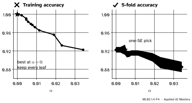
ML02.1.4-F4
Wrong beside right. Training accuracy always prefers \(\alpha = 0\), the unpruned tree. Held-out folds show that the first few prunings cost nothing, and the one-standard-error rule picks the simplest tree that is as good as the best.
“Pick \(\alpha\) by the training accuracy.”
Every pruning step removes splits that were chosen to fit the training set, so training accuracy can only fall as \(\alpha\) grows, and it always votes for no pruning. Choose \(\alpha\) by cross-validation on the training set, and keep the test set for the final check (ML01.9).
“The root question tells me the most important feature.”
It tells you the feature that won on this sample. Over 100 bootstrap samples of the same data, five different features won the root, and the most common one won only 42 times. Interpreting a single tree’s structure is risky. Feature importance done properly, by averaging over many trees or by permuting features, is in ML02.2.
“Pruning fixes the instability.”
It helps a little. A pruned tree has fewer splits that can change, but its top splits are just as fragile, because they are still chosen greedily from one sample, and an early change is passed down to every split below it. In the code above, the pruned bootstrap trees ask exactly the same root questions as the full ones, and the variance of their predictions falls only from 0.056 to 0.047. Averaging many trees is the cure (ML02.2).
Check yourself
Recall
1. Why does a fully grown tree reach 100% training accuracy?
Show answer
It keeps splitting until every leaf is pure, so every training point sits in a leaf that answers its own class (unless two identical points have different labels).
2. Write down the cost-complexity criterion and say what each part does.
Show answer
\(R_\alpha(T) = R(T) + \alpha|T|\). \(R(T)\) is the weighted impurity of the leaves, the fit; \(|T|\) is the number of leaves; \(\alpha\) is the price per leaf, which trades fit against size.
3. What is the effective alpha of an internal node?
Show answer
\({\alpha_{\text{eff}}(t)} = {(R(t) - R(T_t))/(|T_t| - 1)}\): the impurity its branch saves per extra leaf, and the price at which collapsing the branch becomes as cheap as keeping it.
4. Which node is pruned first in weakest-link pruning?
Show answer
The internal node with the smallest effective alpha.
5. How was the instability of a tree measured in this lesson?
Show answer
By growing a tree on each of 100 bootstrap samples and computing, for each test point, the variance \({q(1 - q)}\) of the 0/1 predictions, averaged over the test points.
Exercises
1.★ For \(\alpha = 0.1\), compute \(R_\alpha\) for the four trees \(T_0\) to \(T_3\) of the twelve points and check that \(T_1\) is the cheapest.
Show solution
\(T_0\): \({0 + 5(0.1)} = 0.5\). \(T_1\): \({5/36 + 3(0.1)} \approx 0.439\). \(T_2\): \({5/18 + 2(0.1)} \approx 0.478\). \(T_3\): \({1/2 + 0.1} = 0.6\). The smallest is \(T_1\), as it must be, since \(0.1\) lies between \(5/72 \approx 0.069\) and \(5/36 \approx 0.139\).
2.★★ The tree that cuts only the top-right split has 4 leaves and \(R = 1/12\). Show that it is never the cheapest of the five trees, for any \(\alpha \ge 0\).
Show solution
Its cost is \({1/12 + 4\alpha}\). It beats \(T_0\) only if \({1/12 + 4\alpha} < 5\alpha\), that is \(\alpha > 1/12\). It beats \(T_1\) only if \({1/12 + 4\alpha} < {5/36 + 3\alpha}\), that is \({\alpha < 5/36 - 3/36} = 1/18\). No \(\alpha\) is both above \(1/12 \approx 0.083\) and below \(1/18 \approx 0.056\), so at every \(\alpha\) one of \(T_0\) or \(T_1\) is cheaper.
3.★★★ A node \(t\) has a branch with \(|T_t| = 2\) leaves, so it is a single split. Show that its effective alpha equals the split’s weighted impurity decrease, \(\tfrac{n_t}{n}\,\Delta I\).
Show solution
With children \(a\) and \(b\), \(R(T_t) = {\tfrac{n_a}{n} I(a) + \tfrac{n_b}{n} I(b)}\) and \(R(t) = \tfrac{n_t}{n} I(t)\). Then
For the root of the twelve points, \(n_t = n\) and \(\Delta I = 2/9\), which is the last value of the path.
Summary card
Grow big, prune by a price per leaf chosen by cross-validation, and do not trust one tree too much.
ML02.1.4-F1
Deeper fits training, not new data.
Cost.\(R_\alpha(T) = R(T) + \alpha|T|\).
Effective alpha.\({(R(t) - R(T_t))/(|T_t| - 1)}\); prune the smallest first.
Twelve points. Path \(0, 5/72, 5/36, 2/9\) with 5, 3, 2 and 1 leaves.
In code.cost_complexity_pruning_path, then ccp_alpha chosen by cross-validation.
Instability. Bootstrap trees change their root and disagree on many points: variance.
Sources and next steps
Sources. Each was opened and checked against this lesson on 15 November 2026.
T. Hastie, R. Tibshirani and J. Friedman, The Elements of Statistical Learning, 2nd edition, 12th printing. Section 9.2.2: grow a large tree, then prune with the cost-complexity criterion (9.16) by weakest-link pruning, choosing \(\alpha\) by five- or tenfold cross-validation; Section 9.2.3: the misclassification rate is typically used to guide pruning; Section 9.2.4: the instability of trees, an error in the top split propagated to all splits below, and bagging as the remedy; Section 7.10: the one-standard-error rule.
G. James, D. Witten, T. Hastie, R. Tibshirani and J. Taylor, An Introduction to Statistical Learning, 2nd edition. Section 8.1.1: cost complexity (weakest link) pruning, criterion (8.4) and Algorithm 8.1; Section 8.1.4: trees can be very non-robust.
scikit-learn developers, User Guide, Section 1.10.9: Minimal Cost-Complexity Pruning (version 1.9). \(R_\alpha(T)\), the effective alpha of a node, the weakest link, and \(R(T)\) as the total sample-weighted impurity of the leaves; the warning that small variations in the data can give a completely different tree.
scikit-learn developers, Post pruning decision trees with cost complexity pruning. The breast-cancer split with random_state=0, cost_complexity_pruning_path, dropping the last alpha, and the unpruned tree’s 100% training and 88% test accuracy.
Next. Module ML02.2, Bagging and random forests, grows many trees on bootstrap samples and averages them, turning the instability measured here into an advantage.