Give each component a mean vector and a covariance matrix, so that clusters can be tilted ellipses. Derive the M-step in several dimensions, count the parameters of the four covariance types, and choose K and the type by BIC and AIC.
ML03.4.4L2 Intermediate25 minIn review (what this means)
The maths and code on this page are checked by automated tests on every change, but an independent reader has not signed it off yet. Spot a mistake or a confusing step? Tell us.
Write the density of a multivariate Gaussian, compute a Mahalanobis distance, and draw the ellipses of a covariance matrix from its eigenvectors.
Derive the M-step updates for a component’s mean vector and covariance matrix.
Count the parameters of the full, tied, diagonal and spherical covariance types.
Choose the number of components and the covariance type by BIC and AIC, derived as penalised likelihoods.
Fit a mixture in the plane from scratch and with GaussianMixture, reading predict_proba, bic and aic.
The question
k-means cut scikit-learn’s anisotropic blobs the wrong way (ML03.1.4): each blob is a long, tilted cloud, and k-means can only draw round ones. If each mixture component carries its own covariance matrix, can it trace the tilt? And with no labels to check against, how many components should we fit?
From the last lesson
1. Which choice of the distribution \(q\) makes the lower bound touch the log-likelihood?
Show answer
The responsibilities at the current parameters, \({q_{ik} = r_{ik}}\): the E-step.
2. In what limit does EM for a mixture become k-means?
Show answer
When all components share one fixed variance and that variance shrinks to zero: the responsibilities become 0 or 1 for the nearest centre.
Intuition
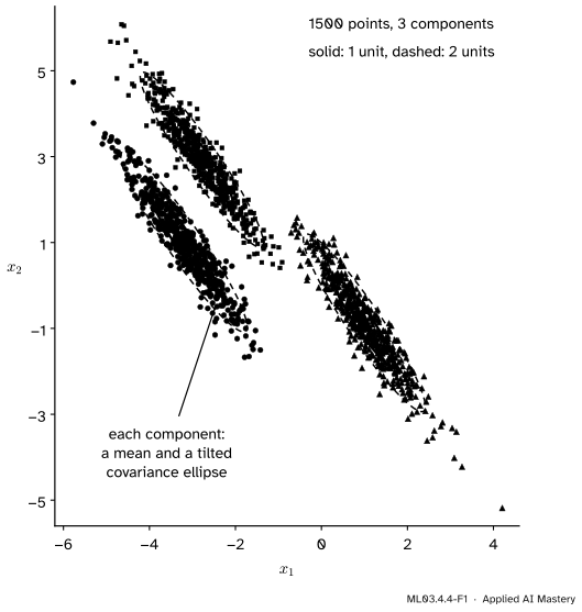
In the plane a Gaussian is a cloud with a centre and a shape. The shape is a covariance matrix\(\mat{\Sigma}\): it says how far the cloud spreads in each direction and how it tilts. Its contours of equal density are ellipses. A mixture in the plane is a few such clouds, each with a weight.
ML03.4.4-F1
A three-component Gaussian mixture fitted to scikit-learn’s anisotropic blobs. Each component’s ellipse follows its cloud’s tilt, so the clusters come out exactly as they were made, where k-means had cut across them.
Nothing in EM changes. The E-step still shares each point between the components by Bayes’ rule; the M-step still refits each component to its share. Only the formulas grow from numbers to vectors and matrices: a mean becomes a mean vector\(\vect{\mu}_k\) and a variance becomes a covariance matrix \(\mat{\Sigma}_k\).
Build it up
Step 1. The multivariate Gaussian. For \(\vect{x}\) in \(\R^d\), the squared Mahalanobis distance from the mean,
With \({d = 1}\) this is the normal density of the earlier lessons, with \({\Delta = \abs{x - \mu}/\sigma}\). This is as far as the module needs the multivariate Gaussian; M07.3 treats it in full.
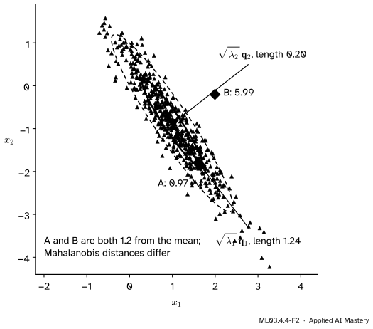
Step 2. The ellipses come from the eigenvectors.\(\mat{\Sigma}\) is symmetric, so it has perpendicular eigenvectors \(\vect{q}_1, \vect{q}_2\) with eigenvalues \({\lambda_1 \ge \lambda_2 > 0}\) (M03.3). The contour \({\Delta = 1}\) is an ellipse whose axes point along the eigenvectors, with half-widths \(\sqrt{\lambda_1}\) and \(\sqrt{\lambda_2}\) (M03.4.4).
ML03.4.4-F2
One component of the fitted mixture. The ellipse’s axes are the eigenvectors of \(\mat{\Sigma}\), scaled by the root eigenvalues. \(A\) and \(B\) are both 1.2 from the mean, but \(A\) lies along the cloud (Mahalanobis distance 0.97) and \(B\) across it (5.99).
Step 3. The E-step is unchanged.\({r_{ik} \propto \pi_k N(\vect{x}_i \mid \vect{\mu}_k, \mat{\Sigma}_k)}\), normalised over \(k\), computed with logarithms as before.
Step 4. The M-step weights vectors and outer products. The mean is the weighted average of the points; the covariance is the weighted average of the outer products \({(\vect{x}_i - \vect{\mu}_k)(\vect{x}_i - \vect{\mu}_k)\T}\), the matrix version of a squared deviation.
The weights and means follow exactly as in ML03.4.2, one coordinate at a time. The covariance is derived in the block below.
Go deeper: deriving the covariance update, entry by entry in the plane
Work with the precision\({\mat{\Lambda} = \mat{\Sigma}^{-1}}\), written \({\begin{bmatrix} a & b \\ b & c \end{bmatrix}}\). Since \({\det \mat{\Sigma} = 1/\det \mat{\Lambda}}\), the terms of \(Q\) that involve component \(k\)’s shape are, with \({\vect{v}_i = \vect{x}_i - \vect{\mu}_k}\),
The fractions \({c/D}\), \({-b/D}\) and \({a/D}\) are exactly the entries of \({\mat{\Lambda}^{-1} = \mat{\Sigma}}\). Setting all three to zero says, entry by entry, \({N_k \mat{\Sigma} = \sum_i r_{ik} \vect{v}_i \vect{v}_i\T}\). The same argument in \(d\) dimensions uses \({\pd{}{\mat{\Lambda}} \ln\det\mat{\Lambda} = \mat{\Lambda}^{-1}}\) for a symmetric \(\mat{\Lambda}\) (Bishop, Appendix C, equation C.28; his section 2.3.4 does the single-Gaussian case).
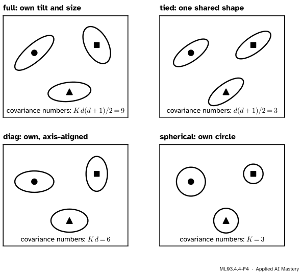
Covariance types. A full covariance in \(d\) dimensions has \({d(d + 1)/2}\) free numbers. With many features that is a lot to estimate per component, so GaussianMixture offers cheaper shapes.
ML03.4.4-F4
The four covariance types, with how many covariance numbers each needs for \({K = 3}\) components in \({d = 2}\) dimensions. Means add \({Kd}\) and weights \({K - 1}\) more.
type
shape
covariance numbers
full
its own matrix
\({K d(d+1)/2}\)
tied
one shared matrix
\({d(d+1)/2}\)
diag
its own diagonal
\({K d}\)
spherical
its own \({\sigma_k^2 \mat{I}}\)
\({K}\)
So the total \(p\) for \({K = 3}\), \({d = 2}\) is \({2 + 6 + 9 = 17}\) for full, 11 for tied, 14 for diagonal and 11 for spherical.
Choosing \(K\) by a penalised likelihood. The maximised log-likelihood \(\hat\ell\) can only grow as components are added, since a mixture with \(K\) components can copy one with \({K - 1}\) by giving a component zero weight. So \(\hat\ell\) alone always asks for more. Two criteria subtract a price for each parameter:
\[
\begin{aligned}
\mathrm{AIC} &= -2\hat\ell + 2p, \\
\mathrm{BIC} &= -2\hat\ell + p \ln n .
\end{aligned}
\]
Smaller is better. AIC estimates how well the model will predict new data: the maximised \(\hat\ell\) is optimistic, because the parameters were fitted to these very points, and for large \(n\) the optimism is about \(p\) (ESL section 7.5). BIC approximates the evidence for the model, the probability of the data averaged over all parameter values; for \({n > 7}\) its price per parameter, \(\ln n\), is the larger, so it prefers simpler models.
Go deeper: where BIC's p ln n comes from
The evidence is \({p(\text{data}) = \int e^{\ell(\theta)} p(\theta)\, d\theta}\) for a prior \(p(\theta)\). Near the maximum \(\hat\theta\), expand \({\ell(\theta) \approx \hat\ell - \tfrac12 (\theta - \hat\theta)\T \mat{H} (\theta - \hat\theta)}\), where \(\mat{H}\) is minus the matrix of second derivatives at \(\hat\theta\). The integral of that Gaussian bump is \({(2\pi)^{p/2} (\det \mat{H})^{-1/2}}\), so
\(\ell\) is a sum of \(n\) terms, so \({\mat{H} \approx n \mat{I}_1}\) for a fixed matrix \(\mat{I}_1\), and \({\ln \det \mat{H} \approx p \ln n + \ln \det \mat{I}_1}\). Keeping only the terms that grow with \(n\), \({\ln p(\text{data}) \approx \hat\ell - \tfrac{p}{2} \ln n}\). Multiply by \(-2\): that is BIC (Bishop 4.137 to 4.139; ESL 7.40). The approximation needs \(n\) large and a well-behaved maximum, which a mixture’s collapsing components can spoil; hence reg_covar.
ML03.4.4-F5
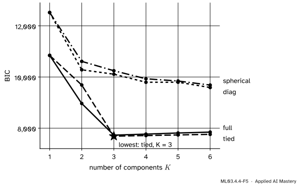
BIC on the anisotropic blobs for each covariance type. The lowest value is three components with one shared covariance: the blobs were made by applying one matrix to round clouds, so they do share a shape. Diagonal and spherical components keep asking for more pieces to tile the tilt.
Worked example
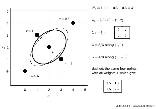
One M-step for one component in the plane. After an E-step, a component has responsibilities 1 for the points \((1, 3)\) and \((3, 1)\) and 0.5 for \((0, 0)\) and \((4, 4)\). Find its new mean and covariance and the axes of its ellipse.
Covariance. The deviations from \((2, 2)\) are \((-1, 1)\), \((1, -1)\), \((-2, -2)\) and \((2, 2)\). The first two have the outer product \({\begin{bmatrix} 1 & -1 \\ -1 & 1 \end{bmatrix}}\) each, the last two \({\begin{bmatrix} 4 & 4 \\ 4 & 4 \end{bmatrix}}\) each, weighted by 0.5. Adding,
and dividing by \({N_k = 3}\) gives \({\mat{\Sigma}_k = \begin{bmatrix} 2 & 2/3 \\ 2/3 & 2 \end{bmatrix}}\).
Ellipse.\({\mat{\Sigma}_k (1, 1) = (8/3)(1, 1)}\) and \({\mat{\Sigma}_k (1, -1) = (4/3)(1, -1)}\). So the ellipse leans along \((1, 1)\) with half-width \({\sqrt{8/3} = 1.63}\), and across it the half-width is \({\sqrt{4/3} = 1.15}\).
ML03.4.4-F3
The worked-example trace. The two heavy points lie across the diagonal, yet the ellipse leans along it, because the half-weighted points are far out. With all four weights equal to 1 the ellipse would be longer and thinner (dashed).
Code
From scratch: EM with full covariances on the anisotropic blobs, started from k-means’s hard labels, then compared with k-means itself by the adjusted Rand index (ML03.10.2; 1 means the same partition as the true blobs).
import numpy as npfrom scipy.special import logsumexpfrom sklearn.cluster import KMeansfrom sklearn.datasets import make_blobsfrom sklearn.metrics import adjusted_rand_scoreX, y = make_blobs(n_samples=1500, random_state=170)X = X @ np.array([[0.60834549, -0.63667341], [-0.40887718, 0.85253229]]) # tilt the blobsdef log_gauss(X, mu, S): D = X - mu _, logdet = np.linalg.slogdet(S) m2 = np.einsum("ni,ij,nj->n", D, np.linalg.inv(S), D) # squared Mahalanobis distancesreturn-0.5* (X.shape[1] * np.log(2* np.pi) + logdet + m2)def e_step(X, pi, mu, S): t = np.log(pi) + np.column_stack([log_gauss(X, m, s) for m, s inzip(mu, S)]) lp = logsumexp(t, axis=1, keepdims=True)return np.exp(t - lp), lp.sum()def m_step(X, r): n_k = r.sum(axis=0) mu = (r.T @ X) / n_k[:, None] S = np.array([(r[:, k, None] * (X - mu[k])).T @ (X - mu[k]) / n_k[k] for k inrange(r.shape[1])])return n_k /len(X), mu, Skm = KMeans(n_clusters=3, n_init=10, random_state=0).fit(X)pi, mu, S = m_step(X, np.eye(3)[km.labels_]) # start from the k-means partitionprevious =-np.inffor it inrange(200): r, ell = e_step(X, pi, mu, S)if ell - previous <1e-8:break previous = ell pi, mu, S = m_step(X, r)print("k-means ARI:", round(adjusted_rand_score(y, km.labels_), 3))print("mixture ARI:", round(adjusted_rand_score(y, r.argmax(axis=1)), 3), " log-likelihood:", round(ell, 1))
The library version, with predict_proba for the soft labels, and BIC and AIC. Both criteria are \({-2\hat\ell}\) plus a penalty, so the parameter count can be read back from them.
from sklearn.mixture import GaussianMixturegm = GaussianMixture(n_components=3, covariance_type="full", random_state=0).fit(X)ell_hat = gm.score(X) *len(X) # score is the mean per pointp_from_bic = (gm.bic(X) +2* ell_hat) / np.log(len(X))print("log-likelihood:", round(ell_hat, 1), " parameters:", round(p_from_bic, 3))print("points with a largest responsibility below 0.99:", int((gm.predict_proba(X).max(axis=1) <0.99).sum()))bic = {kind: [GaussianMixture(k, covariance_type=kind, random_state=0).fit(X).bic(X) for k inrange(1, 7)]for kind in ("full", "tied", "diag", "spherical")}best =min(((v, kind, k +1) for kind, vals in bic.items() for k, v inenumerate(vals)))print("lowest BIC: %.1f for %s with K = %d"% best)
log-likelihood: -3801.3  parameters: 17.0
points with a largest responsibility below 0.99: 6
lowest BIC: 7686.5 for tied with K = 3
Only a handful of the 1500 points are genuinely shared between components. Now BIC and AIC by hand for the six values: one Gaussian (\({p = 2}\)) against two components (\({p = 5}\)).
x6 = np.array([1.0, 2.0, 3.0, 6.0, 8.0, 9.0])ell_1 =-0.5*len(x6) * (np.log(2* np.pi * x6.var()) +1) # one Gaussian at its MLEell_2 =-12.726# where EM settled (ML03.4.2)for name, ell_k, p in (("K = 1", ell_1, 2), ("K = 2", ell_2, 5)):print(name, " BIC:", round(-2* ell_k + p * np.log(6), 2), " AIC:", round(-2* ell_k +2* p, 2))
K = 1  BIC: 33.89  AIC: 34.3
K = 2  BIC: 34.41  AIC: 35.45
Both criteria prefer one Gaussian: 33.89 against 34.41 for BIC, 34.30 against 35.45 for AIC. Six points are too few to pay for three extra parameters, however much they look like two groups.
Explore
Switch the EM stepper in lesson ML03.4.2 to In the plane. With the tilted blobs and \({K = 3}\), step and watch round starting ellipses turn and stretch along the clouds; with the unequal blobs, watch one component stay wide while another shrinks onto the tight group.
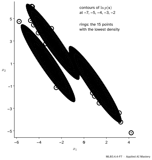
A fitted mixture is also a density. Its log density at any point, score_samples, makes a smooth map, and the points where it is lowest are the least typical. That is the density estimate of ML03.8 and the anomaly score of ML03.9.
ML03.4.4-F7
The fitted mixture as a density. Contours of \({\ln p(\vect{x})}\), and rings on the 1% of points where it is lowest: candidates for anomalies.
Pitfalls
ML03.4.4-F6
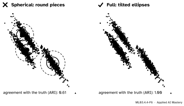
Wrong beside right. Spherical components can only draw circles, so they cut across the tilted clouds as k-means did (adjusted Rand index 0.61). Full covariances follow the tilt (1.00).
“A Gaussian mixture fixes everything that was wrong with k-means.”
Only if its components can take the clusters’ shape. A spherical mixture is soft k-means with unequal sizes, and on tilted clusters it fails the same way. The covariance type is a modelling choice: full is flexible but costly, tied suits clusters of one shape, diagonal and spherical suit clusters aligned with the axes.
“Choose the number of components with the highest log-likelihood.”
\(\hat\ell\) never falls as components are added, and with collapsing components it can grow without limit. Compare by BIC, AIC or held-out log-likelihood instead.
“BIC’s choice is the true number of clusters.”
BIC recovers the true number only with plenty of data drawn from a real mixture of Gaussians, as the scikit-learn guide warns. On the six values it prefers one component. Non-Gaussian clusters, such as moons, are tiled by several Gaussians, and BIC may count the tiles.
Check yourself
Recall
1. Write the squared Mahalanobis distance from \(\vect{x}\) to a component.
Show answer
\({\Delta^2 = (\vect{x} - \vect{\mu})\T \mat{\Sigma}^{-1} (\vect{x} - \vect{\mu})}\): distance in the component’s own units.
2. How do the axes and half-widths of a covariance ellipse come from \(\mat{\Sigma}\)?
Show answer
The axes point along the eigenvectors of \(\mat{\Sigma}\); the half-widths of the \({\Delta = 1}\) ellipse are the square roots of the eigenvalues.
3. Write the M-step update for \(\mat{\Sigma}_k\).
Show answer
The responsibility-weighted average of the outer products, using the new mean:
4. How many covariance numbers does each type need for \(K\) components in \(d\) dimensions?
Show answer
Full \({K d(d+1)/2}\), tied \({d(d+1)/2}\), diagonal \({K d}\), spherical \(K\).
5. Write BIC and AIC, and say which penalises extra parameters more.
Show answer
\({\mathrm{BIC} = -2\hat\ell + p \ln n}\) and \({\mathrm{AIC} = -2\hat\ell + 2p}\), smaller being better. BIC penalises more whenever \({\ln n > 2}\), that is \({n \ge 8}\).
Exercises
1.★ Count the parameters \(p\) of a mixture of \({K = 4}\) components in \({d = 3}\) dimensions for each covariance type.
Show solution
Weights \({K - 1 = 3}\), means \({K d = 12}\), so 15 before the covariances. Full: \({4 \times 6 = 24}\), \({p = 39}\). Tied: 6, \({p = 21}\). Diagonal: \({4 \times 3 = 12}\), \({p = 27}\). Spherical: 4, \({p = 19}\).
2.★★ In the worked example, change both responsibilities of \((0, 0)\) and \((4, 4)\) to 0. Find the new mean and covariance. Which way does the ellipse lean now?
Show solution
\({N_k = 2}\) and the mean is \({\tfrac12 (4, 4) = (2, 2)}\). The deviations \((-1, 1)\) and \((1, -1)\) have the same outer product. Two copies of it, divided by \({N_k = 2}\), give
Its eigenvalues are 2 along \({(1, -1)}\) and 0 along \({(1, 1)}\): the ellipse has collapsed to a line segment across the diagonal. Two points in the plane cannot support a full covariance, which is why reg_covar adds a little to the diagonal.
3.★★★ On the six values, how much higher would the two-component log-likelihood need to be for BIC to prefer two components? And for AIC?
Show solution
BIC prefers two when \({-2\hat\ell_2 + 5 \ln 6 < -2\hat\ell_1 + 2 \ln 6}\), that is \({\hat\ell_2 - \hat\ell_1 > \tfrac32 \ln 6 = 2.688}\). The actual gain is \({\hat\ell_2 - \hat\ell_1 = 2.426}\) (from the unrounded values), short by 0.262. AIC prefers two when \({\hat\ell_2 - \hat\ell_1 > 3}\), short by 0.574. With more points from the same two groups the gain grows in proportion to \(n\), while BIC’s price grows only like \(\ln n\), so two components soon win.
Summary card
In the plane, each component is a mean and an ellipse.
Sources. Each was opened and checked against this lesson on 15 November 2026.
Christopher M. Bishop, Pattern Recognition and Machine Learning, Springer 2006. Section 9.2.2: the covariance update (9.19), “the same form as the corresponding result for a single Gaussian”, weighted by the responsibilities. Appendix C: the derivative of a log-determinant (C.28). Section 4.4.1: the Laplace approximation of the model evidence (4.137) and its rough form, the Bayesian information criterion (4.139).
T. Hastie, R. Tibshirani and J. Friedman, The Elements of Statistical Learning, 2nd edition, corrected 12th printing (2017). Section 7.5: AIC from the optimism of the maximised log-likelihood (7.27) to (7.29). Section 7.7: BIC (7.35), its Laplace-approximation derivation (7.40), and the remark that for \({N > e^2 \approx 7.4}\) it penalises complex models more heavily.
scikit-learn, Gaussian mixture models, User Guide section 2.1: the four covariance types, and BIC recovering the true number of components “only in the asymptotic regime”; the GaussianMixture reference (version 1.9.1) for covariance_type, predict_proba, score_samples, bic and aic; and the k-means assumptions example, source of the anisotropic blobs (make_blobs(n_samples=1500, random_state=170) times a fixed matrix) and of a Gaussian mixture as the remedy.
Next. ML03.5, PCA in depth, returns to the eigenvectors of a covariance matrix, this time to compress the data. Mixtures come back as density estimates in ML03.8, as anomaly scores in ML03.9 and, with BIC, in the judgement of clusterings in ML03.10.