Model data as made by a two-stage story: pick a component, then draw from its bell curve. Write the mixture density, share each point between the components by Bayes’ rule, and see why the log-likelihood has no closed-form maximum.
ML03.4.1L2 Intermediate25 minIn review (what this means)
The maths and code on this page are checked by automated tests on every change, but an independent reader has not signed it off yet. Spot a mistake or a confusing step? Tell us.
Describe the generative story of a Gaussian mixture and write its density as a weighted sum of components.
Compute the responsibility of each component for a point by Bayes’ rule, and read it as a soft cluster label.
Evaluate the log-likelihood of a sample under given mixture parameters, by hand and in NumPy.
Explain why setting the derivative of the log-likelihood to zero gives no closed-form answer.
Sample from a mixture from scratch by picking a component and then drawing from it.
The question
Six measurements came in: 1, 2, 3, 6, 8 and 9. They look like two groups, a low one and a high one. k-means would put 6 in the high group and say nothing more. But 6 sits closer to the gap than any other value. How sure should we be that it belongs with 8 and 9, and can a model say so with a number?
Intuition
Imagine the data were made in two stages. First a coin decides which of two components a point comes from. Then the point is drawn from that component’s bell curve. Each component is a normal distribution with its own centre and width; the coin’s bias says how often each one is used. The result is a Gaussian mixture.
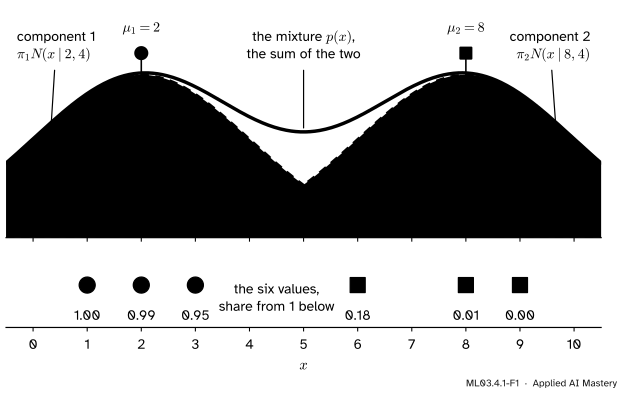
The picture shows the six values with one guess at the two components: centres at 2 and 8, both with variance 4, and a fair coin.
ML03.4.1-F1
A mixture of two Gaussians with weights \(\tfrac12\) and \(\tfrac12\), means 2 and 8 and variance 4. The vermillion mixture density is the sum of the two weighted bumps. Beneath, each value is shaded by its share from component 1: the value 6 is 18% component 1 and 82% component 2.
Two things come out of this one picture. The vermillion curve is the mixture density: the sum of the two dashed bumps, each scaled by its weight. It has two humps, which no single normal curve can have. And every point is shared between the components. The value 1 is almost surely from component 1; the value 6 is mostly from component 2 but not entirely. That share is the responsibility of a component for a point, and it is what makes a mixture a soft clustering: a point is not assigned, it is split.
This is the model behind soft segmentation of customers, speaker models in speaker recognition and many density estimates. The next three lessons fit it; this one sets it up.
Build it up
Step 1. The hidden label. For each point \(x_i\) there is a latent (hidden) variable \(z_i\) that says which component made it: \(z_i = 1\) or \(z_i = 2\). The coin gives \({P(z_i = k) = \pi_k}\), with weights \({\pi_k \ge 0}\) that add to 1.
Step 2. The draw. Given \({z_i = k}\), the point is drawn from \({N(\mu_k, \sigma_k^2)}\). Its density is the normal density of M06.6,
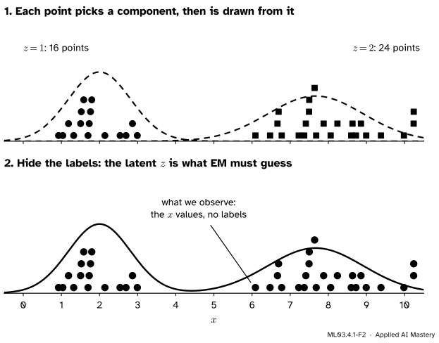
Step 3. We see only \(x\). If we watched the data being made, we would see each \(z_i\) as well (top panel below). In practice we see only the values (bottom panel). Recovering the labels is the clustering problem; recovering the \(\pi_k\), \(\mu_k\) and \(\sigma_k^2\) is the fitting problem.
ML03.4.1-F2
The generative story in two frames. Top: the complete data, where each point’s component \(z\) is known. Bottom: what we actually observe, the values alone. Forty points from the mixture with weights \(\tfrac12, \tfrac12\), means 2 and 7.665 and variances \(\tfrac23\) and 1.565.
Step 4. Add over the hidden label. To get the density of \(x\) alone, add the joint density over both values of \(z\). Writing \({p(x, z = k) = P(z = k)\, p(x \mid z = k)}\) gives the mixture density in the next section.
The formal statement
NoteDefinition: Gaussian mixture
A Gaussian mixture with \(K\) components has weights \({\cparam{\pi_1}, \dots, \cparam{\pi_K}}\) (non-negative, adding to 1), means \(\cparam{\mu_k}\) and variances \(\cparam{\sigma_k^2}\). Its density is
It is a density: each term is non-negative, and integrating term by term gives \({\sum_k \pi_k \cdot 1 = 1}\).
Responsibilities. Bayes’ rule (M06.4) turns the prior \({P(z = k) = \pi_k}\) into a posterior once \(x\) is seen. The posterior is the prior times the likelihood, divided by their sum over all \(k\):
For each point the responsibilities are non-negative and add to 1 over \(k\), because the denominator is the sum of the numerators.
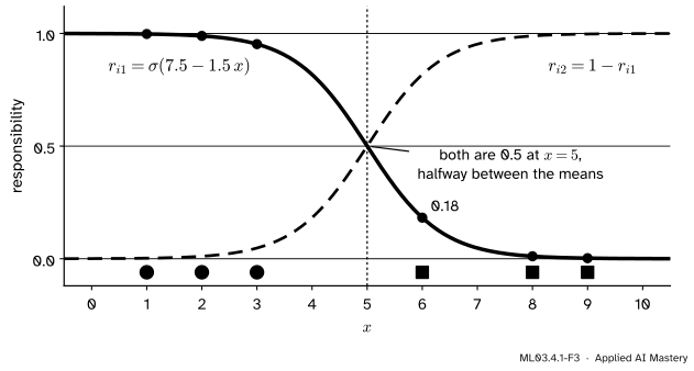
Equal weights and variances give a logistic curve. With two components, \({\pi_1 = \pi_2}\) and \({\sigma_1^2 = \sigma_2^2 = \sigma^2}\), divide the top and bottom of \(r_{i1}\) by the top. The weights and the constants \(1/\sqrt{2\pi\sigma^2}\) cancel, leaving
That is the sigmoid \(\sigma(a)\) of logistic regression (ML01.6). For the starting values, \({(x - 8)^2 - (x - 2)^2 = 60 - 12x}\) and \({2\sigma^2 = 8}\), so
\[
a = \frac{60 - 12x}{8} = 7.5 - 1.5\,x .
\]
ML03.4.1-F3
With equal weights and variances, the responsibility of component 1 is a logistic curve in \(x\). It is \(\tfrac12\) halfway between the means and falls fastest there. The value 6 sits on the steep part, at 0.18.
The log-likelihood. For independent points the likelihood is a product of the densities, so its logarithm (S02.3) is a sum:
Why there is no closed form. Differentiate \(\ell\) with respect to one mean, \(\mu_k\). Every logarithm in the sum depends on \(\mu_k\), but inside each one only the \(k\)th term does. The derivative of a logarithm is the derivative of its argument over the argument, and the chain rule on the exponent of the normal density gives
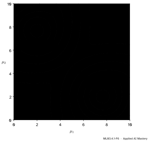
It looks like an answer, a weighted mean, but it is not one: the weights \(r_{ik}\) themselves depend on \(\mu_k\). The equation chases its own tail. The root of the trouble is the logarithm of a sum. With one Gaussian the logarithm undoes the exponential and leaves a quadratic; with a sum inside, it cannot. The surface below shows a second difficulty: the best answer is not unique.
ML03.4.1-F6
The negative log-likelihood of the six values over the two means, with both variances fixed at 1. There are two equally deep valleys, at about \((2, 7.67)\) and \((7.67, 2)\): swapping the components’ names gives the same fit. No single formula picks one out.
Worked example
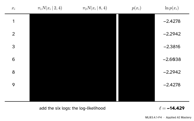
Find the log-likelihood of the six values under the start \({\pi = (\tfrac12, \tfrac12)}\), \({\mu = (2, 8)}\), \({\sigma^2 = (4, 4)}\), and share the value 6 between the components.
With \({\sigma^2 = 4}\) the constant is \({1/\sqrt{8\pi} = 0.19947}\). For \({x = 1}\), the first component gives
and the second gives \({0.5 \times 0.19947\, e^{-49/8} = 0.00022}\). Their sum is the mixture density \({p(1) = 0.08823}\), and \({\ln p(1) = -2.4278}\). The same three steps for every value fill the table.
ML03.4.1-F4
The worked-example trace. Each row adds the two weighted components to get \(p(x_i)\); the logs of the six densities add to the log-likelihood \({\ell = -14.429}\).
Rows 1 and 9 match, and so do rows 2 and 8. With equal weights and variances, a value one unit from one mean scores exactly what a value one unit from the other mean scores, and 1 is one unit from 2 just as 9 is one unit from 8. Adding the last column,
For the value 6 the responsibility of component 1 is the first column over the fourth: \({r_{41} = 0.01350 / 0.07399 = 0.1824}\). The logistic form agrees: \({a = 7.5 - 1.5 \times 6 = -1.5}\) and \({\sigma(-1.5) = 1/(1 + e^{1.5}) = 0.1824}\). So 6 is about 18% component 1 and 82% component 2, the shares printed under the anchor picture.
Code
From scratch first: the normal density, the table of weighted components, the log-likelihood and the responsibilities.
import numpy as npx = np.array([1.0, 2.0, 3.0, 6.0, 8.0, 9.0])pi, mu, var = np.array([0.5, 0.5]), np.array([2.0, 8.0]), np.array([4.0, 4.0])def normal(x, mu, var):return np.exp(-(x - mu) **2/ (2* var)) / np.sqrt(2* np.pi * var)table = pi * normal(x[:, None], mu, var) # n by K: pi_k N(x_i | mu_k, var_k)p = table.sum(axis=1) # the mixture density at each pointell = np.log(p).sum()r = table / p[:, None] # responsibilities, rows add to 1print("p(x_i):", p.round(5))print("log-likelihood:", round(ell, 3))print("r_i1:", r[:, 0].round(4))
Sampling follows the story exactly: pick each \(z_i\) with probabilities \(\pi\), then draw from the chosen normal.
rng = np.random.default_rng(0)n =100_000z = rng.choice(2, size=n, p=pi) # step 1: which componentdraws = rng.normal(mu[z], np.sqrt(var[z])) # step 2: a draw from itprint("share from component 1:", round(np.mean(z ==0), 3))print("sample mean and variance:", round(draws.mean(), 2), round(draws.var(), 2))
share from component 1: 0.501
sample mean and variance: 5.0 13.05
The sample mean is close to 5 and the variance close to 13, not 4: the spread between the two centres adds to the spread within each (exercise 3). Now the library check. SciPy has the normal density, and logsumexp adds probabilities that are stored as logarithms, which the next lesson needs.
from scipy.stats import normfrom scipy.special import logsumexplog_table = np.log(pi) + norm.logpdf(x[:, None], loc=mu, scale=np.sqrt(var))print("log-likelihood via SciPy:", round(logsumexp(log_table, axis=1).sum(), 3))
log-likelihood via SciPy: -14.429
Note that norm takes the standard deviation as scale, not the variance.
Explore
The module’s interactive, the EM stepper, lives in the next lesson. There you can start from these exact values and press E-step: the six points take the shades of the anchor figure.
Pitfalls
ML03.4.1-F5
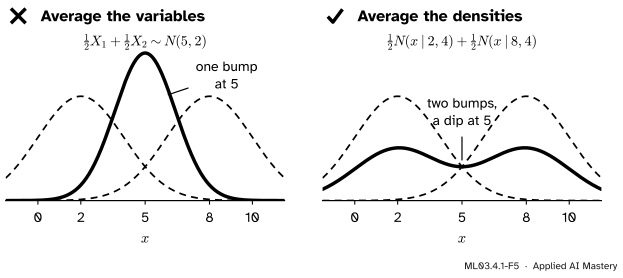
Wrong beside right. Averaging two normal variables gives another normal with one bump. A mixture averages the densities, and keeps both bumps.
“A mixture of two normals is the average of the two normals.”
It is the average of the two densities, not of the two random numbers. If \({X_1 \sim N(2, 4)}\) and \({X_2 \sim N(8, 4)}\) are independent, then \({\tfrac12 X_1 + \tfrac12 X_2}\) is normal with mean 5 and variance \({\tfrac14 \cdot 4 + \tfrac14 \cdot 4 = 2}\): one bump. A mixture instead chooses one of the two and reports it, so its density has two bumps.
“Responsibilities are probabilities, so a point’s responsibilities must add to 1 over the points.”
They add to 1 over the components for each point: the point has to come from somewhere. Summed over the points, \({\sum_i r_{ik}}\) is an effective number of points that component \(k\) explains, and the next lesson calls it \(N_k\).
“A density value above 1 is a mistake.”
A density is not a probability. A narrow component can have a density far above 1 at its centre: \({N(0 \mid 0, 0.01) = 3.99}\). Only the area under a density must be at most 1. This matters in lesson ML03.4.3, where a component that shrinks onto one point drives its density, and the likelihood, to infinity.
Check yourself
Recall
1. Describe the two stages of the generative story of a Gaussian mixture.
Show answer
First pick a component \(k\) with probability \(\pi_k\). Then draw \(x\) from that component’s normal distribution \({N(\mu_k, \sigma_k^2)}\).
2. Write the density of a mixture of \(K\) Gaussians.
Show answer
\({p(x) = \sum_{k=1}^{K} \pi_k N(x \mid \mu_k, \sigma_k^2)}\), with weights \({\pi_k \ge 0}\) that add to 1.
3. What is the responsibility \(r_{ik}\), and which rule gives it?
Show answer
The posterior probability that point \(i\) came from component \(k\), by Bayes’ rule: the weighted density \({\pi_k N(x_i \mid \mu_k, \sigma_k^2)}\) divided by its sum over all the components.
4. What is the log-likelihood of the six values under the starting values?
Show answer
\({\ell = -14.429}\), the sum of the six values of \({\ln p(x_i)}\).
5. Why does setting \({\pd{\ell}{\mu_k} = 0}\) not give a closed-form answer?
Show answer
It gives \({\mu_k = \sum_i r_{ik} x_i / \sum_i r_{ik}}\), but the weights \(r_{ik}\) depend on \(\mu_k\) (and on all the other parameters), so the equation is circular. The cause is the logarithm of a sum in \(\ell\).
Exercises
1.★ Under the starting values, find the responsibility of component 1 for the value \({x = 5}\) and for \({x = 4}\).
Show solution
With equal weights and variances, \({r_{i1} = \sigma(7.5 - 1.5x)}\). At \({x = 5}\), \({a = 0}\) and \({r = \sigma(0) = 0.5}\): 5 is halfway between the means. At \({x = 4}\), \({a = 1.5}\) and \({r = 1/(1 + e^{-1.5}) = 0.8176}\).
2.★★ Keep the means at 2 and 8 and both variances at 4, but change the weights to \({\pi = (0.2, 0.8)}\). Where is a point now shared equally between the two components?
Show solution
Equal shares mean \({\pi_1 N(x \mid 2, 4) = \pi_2 N(x \mid 8, 4)}\). Take logarithms; the constants \(1/\sqrt{8\pi}\) cancel:
Multiply by 8 and rearrange: \({(x - 8)^2 - (x - 2)^2 = 8 \ln 4}\), that is \({60 - 12x = 11.09}\), so \({x = 4.08}\). The heavier component 2 claims more of the line, and the equal-share point moves from 5 towards the lighter component.
3.★★★ Show that a two-component mixture has mean \({\bar\mu = \pi_1\mu_1 + \pi_2\mu_2}\) and variance
which gives the result: the average spread within the components plus the spread of their centres. For the start, \({\bar\mu = 5}\) and the variance is \({4 + \tfrac12 \cdot 9 + \tfrac12 \cdot 9 = 13}\), matching the sample’s 13.
Summary card
A mixture adds weighted bumps, and shares every point between them.
ML03.4.1-F1
Weighted bumps, summed; points shared.
Story.\({z \sim \pi}\), then \({x \mid z = k \sim N(\mu_k, \sigma_k^2)}\).
Log-likelihood.\({\ell = \sum_i \ln p(x_i)}\): a log of a sum, with no closed-form maximum.
Sources and next steps
Sources. Each was opened and checked against this lesson on 15 November 2026.
Christopher M. Bishop, Pattern Recognition and Machine Learning, Springer 2006. Section 9.2: the mixture density (9.7), the latent variable and the sum over it (9.12), the responsibilities (9.13). Section 9.2.1: the log-likelihood (9.14), the remark that the sum inside the logarithm means “we will no longer obtain a closed form solution”, and the \(K!\) equivalent solutions from swapping labels.
T. Hastie, R. Tibshirani and J. Friedman, The Elements of Statistical Learning, 2nd edition, corrected 12th printing (2017). Section 8.5.1: the two-component model as a generative story (8.36), its density (8.37) and log-likelihood (8.39), and the difficulty of maximising it directly “because of the sum of terms inside the logarithm”.
scikit-learn, Gaussian mixture models, User Guide section 2.1, for the library’s description of mixtures as soft, probabilistic clustering; the class itself is used from the next lesson on.