Forbid negative entries in both factors and a factorisation turns into parts that only add up. Derive Lee and Seung’s multiplicative updates from gradient descent, run one by hand, and find sports and baking topics and pen strokes.
ML03.7.2L2 Intermediate25 minIn review (what this means)
The maths and code on this page are checked by automated tests on every change, but an independent reader has not signed it off yet. Spot a mistake or a confusing step? Tell us.
State the non-negative matrix factorisation problem and explain why non-negative factors read as additive parts.
Derive the multiplicative updates for the squared error as gradient descent with a step chosen for each entry.
Carry out one multiplicative update by hand and check that the error falls.
Fit NMF from scratch and with sklearn.decomposition.NMF, and explain why its factors are not unique.
The question
The last lesson’s factors said that a document is “all words, plus sports, minus baking”, and its rank-2 reconstruction claimed that d1 contains \({-0.12}\) of the word “oven”. Can we keep the idea of a thin matrix times a wide one but insist that documents are built only by adding parts, never by taking words away?
From the last lesson
1. What is the smallest squared error of a rank-2 product for the corpus, and where does it come from?
Show answer
5.692, the sum of the discarded squared singular values \({3.20 + 1.54 + 0.73 + 0.22 + 0}\) (Eckart and Young).
2. How is a new document placed in the LSA plane?
Show answer
By folding in: multiply its count vector by \(\mat{U}_2\T\), that is, take its dot product with the first two left singular vectors.
Intuition
Require every entry of \(\mat{W}\) and of \(\mat{H}\) to be zero or more. Then each column of \(\mat{W}\) is a set of words with non-negative weights: a part. Each document is a sum of parts with non-negative amounts, so a part can be switched on or left out, but never subtracted.
ML03.7.2-F1
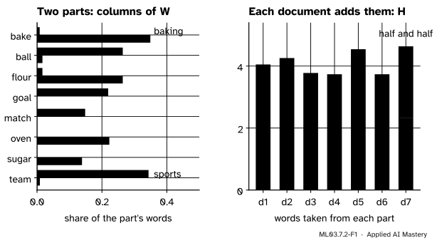
Non-negative factors of the corpus with rank 2. Each column of \(\mat{W}\) (scaled to sum to 1) is a part, here a sports part and a baking part. Each document takes some words from each part; d7 takes about 2.3 from each.
Nothing told the method which words go together. The constraint alone produced two parts that a person would name “sports” and “baking”. This is non-negative matrix factorisation (NMF), and the effect is called a parts-based representation: Lee and Seung contrasted it with PCA, which builds data from directions that cancel each other, and with clustering, where each example takes exactly one prototype.
Build it up
Step 1. The problem. Given a non-negative \({V \times D}\) matrix \(\mat{X}\) and a rank \(q\), solve
Step 2. No formula, so iterate. The SVD answer of the last lesson breaks the constraint, and no closed form is known. For fixed \(\mat{W}\) the error is a convex bowl in \(\mat{H}\), and for fixed \(\mat{H}\) a bowl in \(\mat{W}\), but it is not convex in both at once. So we alternate: improve \(\mat{H}\) with \(\mat{W}\) fixed, then \(\mat{W}\) with \(\mat{H}\) fixed, and accept a local minimum.
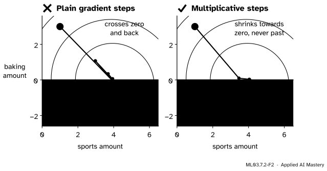
Step 3. Plain gradient steps can cross zero. Take one document, d1, and fix \(\mat{W}\) to the two parts. The error is a bowl over the two amounts. Gradient descent with a fixed step walks downhill, but nothing stops a step from landing on a negative amount.
ML03.7.2-F2
The same bowl, two kinds of step from the same start. A fixed gradient step overshoots into negative amounts; the multiplicative step multiplies the amount by a positive factor, so it can shrink towards zero but never crosses it.
Step 4. Pick a step for each entry. A gradient step can use a different step size for every entry. Lee and Seung chose the one size that cancels the subtraction, so that the step becomes a multiplication by a positive factor. The derivation follows.
The formal statement
The gradient. Write \({\mat{R} = \mat{X} - \mat{W}\mat{H}}\). Changing \(\mat{H}\) by a small \({\delta\mat{H}}\) changes the product by \({\mat{W}\,\delta\mat{H}}\), so to first order
Started from positive matrices, every entry stays non-negative, and the squared error never increases.
The update for \(\mat{W}\) is the twin: the same argument applied to \({\mat{X}\T \approx \mat{H}\T\mat{W}\T}\).
Read the factor as what the data asks for over what the model already gives. When the model under-supplies a part, the factor is above 1 and the amount grows; when it over-supplies, the factor is below 1 and the amount shrinks. The factor is never negative, so a positive entry stays positive. A zero stays zero for ever, which is why a start with zeros in it is a bad idea. If \({\mat{X} = \mat{W}\mat{H}}\) exactly, every factor is 1 and nothing moves.
ML03.7.2-F3
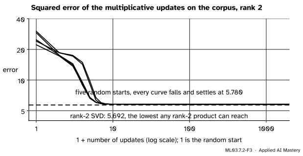
Five random starts on the corpus. The error only falls, and every start settles at 5.780, just above the SVD’s 5.692. The constraint raises the error by 1.5 percent and buys readable parts.
Go deeper: why the error never rises: the auxiliary function
Lee and Seung’s proof works one column \(\vect{h}\) of \(\mat{H}\) at a time, with \({F(\vect{h}) = \tfrac12\norm{\vect{x} - \mat{W}\vect{h}}^2}\). A function \({G(\vect{h}, \vect{h}')}\) is an auxiliary function for \(F\) if \({G(\vect{h}, \vect{h}') \ge F(\vect{h})}\) for all \(\vect{h}\) and \({G(\vect{h}, \vect{h}) = F(\vect{h})}\). Then moving to the minimiser of \({G(\cdot, \vect{h}^t)}\) cannot raise \(F\):
\(F\) is exactly quadratic, with curvature matrix \(\mat{W}\T\mat{W}\). Replace that curvature by a diagonal matrix \(\mat{K}\) with \({K_{aa} = (\mat{W}\T\mat{W}\vect{h}^t)_a / h^t_a}\):
\(G\) touches \(F\) at \({\vect{h} = \vect{h}^t}\). It lies above \(F\) everywhere if \({\mat{K} - \mat{W}\T\mat{W}}\) is positive semidefinite; rescaling it to \({M_{ab} = h^t_a (\mat{K} - \mat{W}\T\mat{W})_{ab} h^t_b}\) and expanding gives
Because \(\mat{K}\) is diagonal, \(G\) is minimised entry by entry: setting its gradient to zero gives \({h_a = h^t_a - (\nabla F)_a / K_{aa}}\), which simplifies to the multiplicative update. The details are Lemmas 1 and 2 of the paper.
Worked example
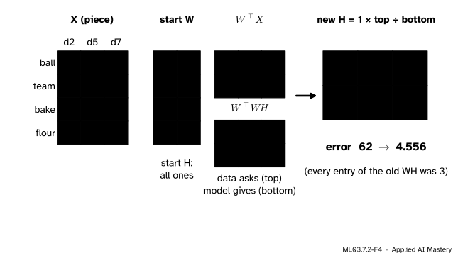
One update of \(\mat{H}\) by hand. Use the small piece of the corpus: words ball, team, bake, flour (rows) in documents d2, d5, d7 (columns), with \({q = 2}\). Start from
and \(\mat{H}\) all ones. Every entry of the starting product is \({2 + 1 = 3}\), so the starting error is the sum of \({(x - 3)^2}\) over the twelve cells, row by row:
One multiplicative update of \(\mat{H}\). Each new entry is the old one (1) times what the data asks for over what the model gives.
What the data asks for. Row 1 of \(\mat{W}\T\) is \({(2, 2, 1, 1)}\), so the first row of \(\mat{W}\T\mat{X}\) is \({(2 + 4,\; 2 + 1,\; 2 + 2 + 1 + 1)}\), which is \({(6, 3, 6)}\). Row 2, \({(1, 1, 2, 2)}\), gives \({(1 + 2,\; 4 + 2,\; 1 + 1 + 2 + 2)}\), which is \({(3, 6, 6)}\).
What the model gives.\({\mat{W}\T\mat{W}}\) has entries \({4 + 4 + 1 + 1 = 10}\) on the diagonal and \({2 + 2 + 2 + 2 = 8}\) off it. Times \(\mat{H}\) of ones, every entry is \({10 + 8 = 18}\).
The update. Each entry of \(\mat{H}\) becomes \({1 \times (\text{top}) / 18}\):
d2 now leans to part 1 and d5 to part 2, while d7 takes both equally.
The new error. The new product has rows \({(5/6, 2/3, 1)}\) for ball and team and \({(2/3, 5/6, 1)}\) for bake and flour. The squared errors are \({17/36}\) for ball, \({65/36}\) for team, \({65/36}\) for bake and \({17/36}\) for flour, in total \({164/36 = 4.556}\). One step took the error from 62 to 4.556. The matching update of \(\mat{W}\) takes it to 3.803, and 500 steps to 0.245.
Code
From scratch on the corpus, keeping the error after every pair of updates.
import numpy as npdocs = ["ball goal team goal", "team match ball team", "goal match team ball","flour sugar bake oven", "bake oven flour bake", "sugar flour bake oven","team bake ball flour"]words =sorted({w for d in docs for w in d.split()})X = np.array([[d.split().count(w) for d in docs] for w in words], dtype=float)def nmf(X, q, steps, seed=0, eps=1e-12): rng = np.random.default_rng(seed) W = rng.uniform(0.1, 1.0, (X.shape[0], q)) H = rng.uniform(0.1, 1.0, (q, X.shape[1])) errors = []for _ inrange(steps): H *= (W.T @ X) / (W.T @ W @ H + eps) W *= (X @ H.T) / (W @ H @ H.T + eps) errors.append(((X - W @ H) **2).sum())return W, H, np.array(errors)W, H, errors = nmf(X, 2, 2000)scale = W.sum(axis=0) # make each part a set of shares ...parts, amounts = W / scale, H * scale[:, None] # ... and move the scale into Hsvd_floor = (np.linalg.svd(X, compute_uv=False)[2:] **2).sum()for k inrange(2): top = [words[i] for i in np.argsort(-parts[:, k])[:4]]print(f"part {k +1}: {top}")print("d7 takes", amounts[:, 6].round(2), "words from the two parts")print(f"error {errors[-1]:.3f} (SVD floor {svd_floor:.3f}); ever rose: {bool(np.any(np.diff(errors) >1e-9))}")
part 1: ['team', 'ball', 'goal', 'match']
part 2: ['bake', 'flour', 'oven', 'sugar']
d7 takes [2.32 2.32] words from the two parts
error 5.780 (SVD floor 5.692); ever rose: False
The library. NMF takes examples as rows, so we pass \({\mat{X}\T}\): its fit_transform returns the document amounts and components_ the parts. The start init="nndsvda" comes from an SVD with zeros filled in, since multiplicative updates cannot move a zero. beta_loss="kullback-leibler" (with solver="mu") swaps the squared error for a divergence suited to counts; the next lesson shows what it means.
from sklearn.decomposition import NMFmodel = NMF(n_components=2, init="nndsvda", max_iter=2000, tol=1e-10, random_state=0)doc_amounts = model.fit_transform(X.T) # 7 x 2print("squared error:", round(model.reconstruction_err_ **2, 3))kl = NMF(n_components=2, init="nndsvda", beta_loss="kullback-leibler", solver="mu", max_iter=5000, tol=1e-12, random_state=0)A = kl.fit_transform(X.T)words_from_part = A * kl.components_.sum(axis=1) # scale each part to sum to 1print("KL loss, d7 takes", words_from_part[6].round(3), "words from each part")
squared error: 5.78
KL loss, d7 takes [2. 2.] words from each part
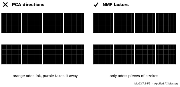
On images the same constraint finds strokes. Fitted to the 1797 digits of load_digits, each of 16 factors lights up a short piece of pen stroke, while PCA’s directions are patterns of light and dark that cancel.
from sklearn.datasets import load_digitsdigits = load_digits().data # 1797 x 64, values 0 to 16strokes = NMF(n_components=16, init="nndsvda", max_iter=500, random_state=0).fit(digits)share_zero = (strokes.components_ <1e-3).mean()print(f"{share_zero:.0%} of the factor pixels are (nearly) zero")
75% of the factor pixels are (nearly) zero
ML03.7.2-F6
Factors of the handwritten digits. PCA’s directions use cancellation; NMF’s factors are mostly blank, each holding one piece of a stroke, and a digit is a sum of a few of them.
Explore
ML03.7-X1
Factor explorer
The corpus’s 8 by 7 count matrix beside its two factors. Choose the rank and switch between the truncated SVD and NMF; for NMF, step the multiplicative updates or play them. Compare the error, the top words of each factor and the purple negative cells of the SVD.
Pitfalls
ML03.7.2-F5
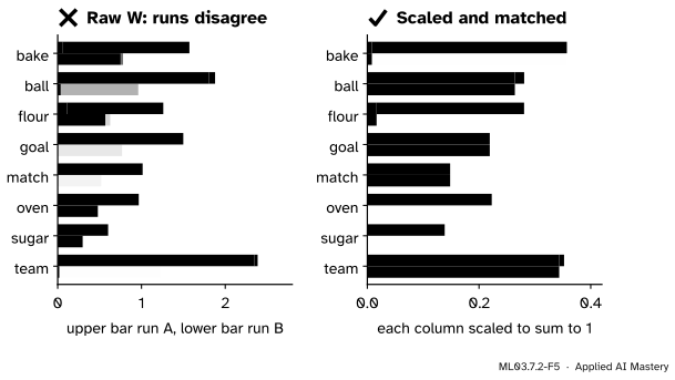
Wrong beside right. Two fits with different starts give different numbers in \(\mat{W}\). Scale each column to sum to 1 and match the parts, and they agree.
“Two runs gave different W, so one of them is wrong.”
For any diagonal matrix \(\mat{D}\) with positive entries, \({\mat{W}\mat{D}}\) and \({\mat{D}^{-1}\mat{H}}\) are non-negative and have the same product, and the parts can come out in any order. Fix the scale (each column of \(\mat{W}\) summing to 1) and match the parts before comparing. Beyond scaling and order, NMF can also stop at different local minima from different starts, so on real data compare several runs.
“NMF fits better than the SVD because it is cleverer.”
It cannot. The SVD gives the smallest error of any rank-\(q\) product; NMF searches a smaller set. On the corpus the costs are 5.692 against 5.780 at rank 2 and 2.495 against about 2.60 at rank 3. You give up a little fit to gain parts you can read.
“Start the updates from the SVD’s factors with the negatives set to zero.”
A zero entry is multiplied by a factor and stays zero, so every part that starts with zeros keeps them. That is why scikit-learn’s guide prefers "nndsvda", which fills those zeros with the mean of the data, when the multiplicative solver is used.
Check yourself
Recall
1. What does the non-negativity constraint change about how a document is built from parts?
Show answer
Parts can only be added in non-negative amounts, never subtracted, so each part reads as a group of words that appear together.
2. Write the multiplicative update for \(\mat{H}\).
Show answer
\({\mat{H} \leftarrow \mat{H} \circ (\mat{W}\T\mat{X}) / (\mat{W}\T\mat{W}\mat{H})}\), entry by entry.
3. Which step size turns gradient descent on \(h_{kd}\) into that update?
Show answer
\({\eta_{kd} = h_{kd} / \big(2(\mat{W}\T\mat{W}\mat{H})_{kd}\big)}\), which cancels the old value and leaves only the multiplication.
4. Why does an entry that starts at zero never move?
Show answer
Each update multiplies the entry by a factor, and zero times anything is zero.
5. On the corpus at rank 2, how do the NMF and SVD errors compare, and why can NMF not win?
Show answer
5.780 against 5.692. The SVD’s product is the best of all rank-2 products; NMF’s are a subset.
Exercises
1.★ Continue the worked example. With the new \(\mat{H}\), the first row of \({\mat{X}\mat{H}\T}\) (ball) is \({(2/3, 1/2)}\) and the first row of \({\mat{W}\mat{H}\mat{H}\T}\) is \({(26/36, 25/36)}\). Find the new first row of \(\mat{W}\).
Show solution
Multiply the old row \({(2, 1)}\) by the ratios entry by entry:
2.★★ Show that for one column \({\vect{x} \ge 0}\) and one part \({\vect{w} \ge 0}\) (\({q = 1}\), \(\vect{w}\) fixed), a single multiplicative update from any \({h > 0}\) lands on the best non-negative \(h\).
Show solution
The update replaces \(h\) by \({h\,\vect{w}\T\vect{x} / (\vect{w}\T\vect{w}\,h)}\), which is \({\vect{w}\T\vect{x} / \vect{w}\T\vect{w}}\): the old \(h\) cancels. The error \({\norm{\vect{x} - h\vect{w}}^2}\) is a parabola in \(h\) with derivative \({2(h\,\vect{w}\T\vect{w} - \vect{w}\T\vect{x})}\), zero at that same value. It is non-negative because \(\vect{w}\) and \(\vect{x}\) are, so it is the best non-negative \(h\) too.
3.★★★ Suppose \(\mat{W}\) and \(\mat{H}\) are positive and \({\mat{W}\mat{H} = \mat{X}}\) exactly. Show that both updates leave them unchanged. Then show that the converse fails: a fixed point of the updates need not have zero error.
Show solution
If \({\mat{W}\mat{H} = \mat{X}}\) then \({\mat{W}\T\mat{W}\mat{H} = \mat{W}\T\mat{X}}\), so every factor in the \(\mat{H}\) update is 1, and likewise \({\mat{W}\mat{H}\mat{H}\T = \mat{X}\mat{H}\T}\) for \(\mat{W}\). For the converse, run the updates on the corpus with \({q = 2}\): they stop changing at error 5.780, which is not zero (and cannot be, since no rank-2 product has error below 5.692). At such a point every positive entry has a zero gradient, which is a stationary point of the constrained problem, not an exact fit.
Summary card
Non-negative factors are parts that only add.
ML03.7.2-F1
Sports and baking, found by the constraint.
Problem: minimise \({\norm{\mat{X} - \mat{W}\mat{H}}_F^2}\) with \({\mat{W}, \mat{H} \ge 0}\).
Updates: each entry of \(\mat{H}\) is multiplied by \({(\mat{W}\T\mat{X})}\) over \({(\mat{W}\T\mat{W}\mat{H})}\), and the twin for \(\mat{W}\).
Never unique:\({\mat{W}\mat{D}}\), \({\mat{D}^{-1}\mat{H}}\) fit as well; scale and match parts.
Sources and next steps
Sources. Each was opened and checked against this lesson on 15 November 2026.
D. D. Lee and H. S. Seung, Algorithms for Non-negative Matrix Factorization, NIPS 13 (2001). Section 1 contrasts PCA’s cancellations and clustering’s single prototypes with the parts representation of NMF; section 2 reads each column as a combination of the columns of \(\mat{W}\); Theorem 1 (equation 4) gives the updates; section 5 (equations 6 and 7) derives them as rescaled gradient descent; section 6 (Lemmas 1 and 2) gives the auxiliary-function proof.
scikit-learn, Non-negative matrix factorization, User Guide section 2.5.7: NNDSVDa fills zeros with the mean of the data and is preferred with the multiplicative solver, which cannot update zeros; that solver can minimise the Kullback-Leibler divergence.
scikit-learn, NMF: beta_loss is used only by the "mu" solver, and reconstruction_err_ is the Frobenius norm of \({\mat{X} - \mat{W}\mat{H}}\), not its square.