Where Lloyd’s algorithm starts decides where it stops. Seed it with k-means++, which spreads the first centres out, run it from several starts, read the elbow of J against K for a bend rather than a minimum, and quantise the colours of a photo with MiniBatchKMeans.
ML03.1.3L2 Intermediate25 minIn review (what this means)
The maths and code on this page are checked by automated tests on every change, but an independent reader has not signed it off yet. Spot a mistake or a confusing step? Tell us.
Show with repeated runs that random starts can leave k-means in poor local minima.
Carry out k-means++ seeding by hand and in code, and state its guarantee on the expected J.
Explain why several starts are run and the lowest J kept, and what scikit-learn’s KMeans does by default.
Read a plot of J against K for a bend, and explain why its minimum is useless for choosing K.
Count the cost n K d of one round of Lloyd’s algorithm and use MiniBatchKMeans to quantise an image.
The question
Run k-means twice on the same data with the same \(K\) and you can get two different answers, one of them far worse than the other. Which start should you trust, how can a start be chosen so that bad answers are rare, and how many clusters should you ask for in the first place?
From the last lesson
1. Why does Lloyd’s algorithm always stop?
Show answer
While the assignment keeps changing, \(J\) strictly falls, so no assignment can come back, and there are only finitely many assignments.
2. Does it always stop at the lowest possible \(J\)?
Show answer
No. It stops at a local minimum. On the nine points, the start \((2, 2)\) and \((7, 6)\) stops at \(J = 14\) instead of \(10.8\).
Intuition
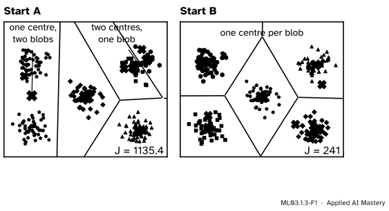
Take 250 points in five well-separated blobs and ask for \(K = 5\). Start Lloyd’s algorithm from five data points picked at random. Sometimes two starting centres land in the same blob, and none lands in another. Lloyd’s algorithm only makes local repairs, so it cannot fix that.
ML03.1.3-F1
The same data, the same \(K\), two starts. Start A leaves one centre between two blobs and two centres inside one blob, and stops at \(J = 1135.4\). Start B ends with one centre per blob and \(J = 241\).
Two cures follow. Choose starts that are spread out, so that every blob is likely to get a centre: that is k-means++. And run the algorithm from several starts and keep the run with the lowest \(J\), since \(J\) is exactly the score we want to be small.
Build it up
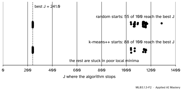
Step 1. Measure how often starts go wrong. Run Lloyd’s algorithm from 100 random starts on the blobs and record where each run stops. The best value, \(J = 240.97\), is one centre per blob.
ML03.1.3-F2
Where Lloyd’s algorithm stops, for 100 starts of each kind on the five blobs. Only 55 random starts reach the best \(J\); 88 of the k-means++ starts do. Every other run is stuck far higher, between about \(J = 1040\) and \(J = 1290\).
Step 2. Spread the starts out. k-means++ picks the first centre at random. Then, for every point, it measures \(D(\vect{x})\), the distance to the nearest centre chosen so far, and draws the next centre with probability proportional to \(D(\vect{x})^2\). A point in a blob that already has a centre is close to it and is rarely drawn; a point in an empty blob is far away and likely to be.
Step 3. Keep the best of several runs. Each run ends at some local minimum. Run several and keep the one with the lowest \(J\). With 55 percent of random runs succeeding here, ten runs all fail with probability about \({0.45^{10}} \approx 0.0003\).
Step 4. Choose K.\(J\) cannot choose \(K\) on its own, because more clusters always fit better. The useful signal is the shape of the curve of \(J\) against \(K\).
The formal statement
Notek-means++ seeding (Arthur and Vassilvitskii, 2007)
Choose the first centre \(\vect{\mu}_1\) uniformly at random from the data points.
For each point, let \(D(\vect{x}_i)\) be the distance to the nearest centre chosen so far. Choose the next centre to be \(\vect{x}_i\) with probability
Repeat step 2 until \(K\) centres are chosen, then run Lloyd’s algorithm from them.
Arthur and Vassilvitskii call this “\(D^2\) weighting”. A point that is already a centre has \(D = 0\), so it is never drawn twice. Their main result bounds what the seeding alone achieves, before Lloyd’s algorithm improves it further.
NoteTheorem (Arthur and Vassilvitskii, Theorem 3.1)
If the centres are chosen by k-means++, the expected value of \(J\) at those centres satisfies
\[
\E[J] \le 8\,(\ln K + 2)\, J_{\text{opt}} ,
\]
where \(J_{\text{opt}}\) is the lowest \(J\) possible with \(K\) clusters.
For \(K = 5\) the factor is \(8\,(\ln 5 + 2) \approx 28.9\). That is a guarantee in the worst case, over every possible data set, and it grows only like \(\ln K\). Random seeding has no such guarantee: Arthur and Vassilvitskii point out natural data sets on which the ratio \(J / J_{\text{opt}}\) that Lloyd’s algorithm reaches from random starts is unbounded.
What scikit-learn does.KMeans(n_clusters=K) uses init="k-means++" and, since version 1.4, n_init="auto". With k-means++ seeding, “auto” means one run; with init="random" it means ten. scikit-learn’s seeding is a greedy k-means++: at each step it draws \({2 + \lfloor \ln K \rfloor}\) candidates by \(D^2\) weighting and keeps the one that lowers \(J\) most. Set n_init to 10 or more yourself when a poor local minimum would be costly.
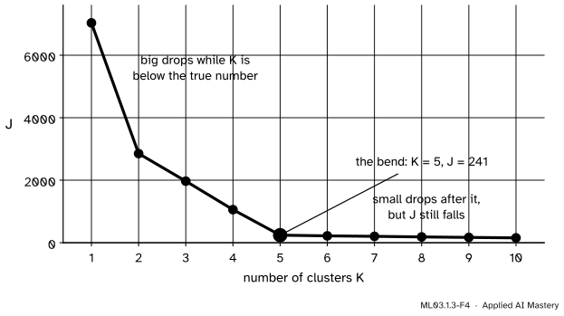
Choosing K: the elbow. Let \(J^*(K)\) be the lowest \(J\) with \(K\) clusters. It can only fall as \(K\) grows: take the best \(K\)-clustering, move one point that does not sit exactly on its centre into a new cluster of its own, and its term drops to zero, so \(J^*(K + 1) < J^*(K)\) whenever some cluster has two different points (Exercise 3). With one cluster per distinct point, \(J = 0\). So the minimum of the curve is always at the largest \(K\) tried and says nothing.
The shape says more. While \(K\) is below the true number of groups, each new cluster splits two real groups apart and \(J\) falls a lot. Past it, each new cluster splits a real group in two and \(J\) falls a little. The elbow is the bend between the two regimes.
ML03.1.3-F4
\(J\) against \(K\) for the five blobs, each from the best of ten runs. \(J\) falls all the way to \(K = 10\), but the bend at \(K = 5\) is where the big drops stop.
Go deeper: the cost of one round, and mini-batches
One assignment step computes the squared distance from each of \(n\) points to each of \(K\) centres, and each squared distance costs about \(d\) multiplications and \(d\) additions. So one round costs on the order of \(n K d\) operations; the update adds only \(n d\). Mini-batch k-means (in scikit-learn, MiniBatchKMeans) assigns and updates using a small random batch of \(b\) points at each step, by default \(b = 1024\), so one step costs about \({b\,K d}\) whatever \(n\) is. The scikit-learn user guide describes its results as generally only slightly worse than the standard algorithm.
Worked example
Seed \(K = 2\) on the nine points with k-means++, after the first centre \((1, 1)\).
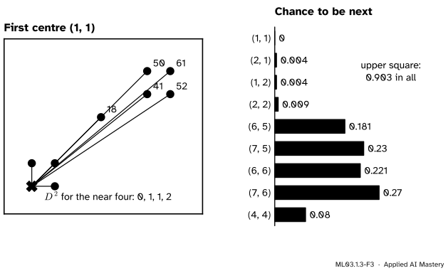
Squared distances. Every point’s \(D^2\) is its squared distance to \((1, 1)\):
Probabilities. Divide each by \(226\). The most likely next centre is \((7, 6)\), with \(61/226 \approx 0.270\). The upper square as a whole gets \(204/226 \approx 0.903\), the bridge point \(18/226 \approx 0.080\) and the rest of the lower square only \(4/226 \approx 0.018\).
ML03.1.3-F3
k-means++ after the first centre \((1, 1)\). Each point’s chance is its \(D^2\) over \(226\). Nine times in ten the second centre lands in the far square, where a second centre belongs.
Where it leads. From \((1, 1)\) every second centre leads Lloyd’s algorithm to \(J = 10.8\), but other first centres are less lucky. Averaging over all nine first centres and every second centre, the chance of ending in the trap \(J = 14\) is about \(0.25\) for k-means++ (between \(0.246\) and \(0.261\), depending on which centre gets a point that is tied between two). For two distinct data points picked uniformly at random it is \(13/36 \approx 0.36\): eleven of the 36 pairs always end in the trap, and four more do so half the time, depending on the order in which the two are listed (last lesson). Better, but not perfect, which is why several runs are still worth it.
Code
k-means++ from scratch, then the 100-start experiment of the figure. The seeds are fixed, so the counts can be reproduced; a different NumPy could shift them by a run or two.
import numpy as npfrom sklearn.datasets import make_blobsdef plusplus(X, K, rng):"""k-means++ seeding: the first centre uniformly, each next one with probability D^2 / sum D^2.""" C = [X[rng.randint(len(X))]]for _ inrange(K -1): D2 = ((X[:, None, :] - np.array(C)[None, :, :]) **2).sum(axis=-1).min(axis=1) C.append(X[rng.choice(len(X), p=D2 / D2.sum())])return np.array(C)def lloyd_end(X, C, rounds=300):"""Run Lloyd's algorithm to the end; return the final J.""" C = np.array(C, dtype=float)for _ inrange(rounds): z = ((X[:, None, :] - C[None, :, :]) **2).sum(axis=-1).argmin(axis=1) new = np.array([X[z == k].mean(axis=0) if np.any(z == k) else C[k] for k inrange(len(C))])if np.allclose(new, C):break C = new z = ((X[:, None, :] - C[None, :, :]) **2).sum(axis=-1).argmin(axis=1)return ((X - C[z]) **2).sum()X, y = make_blobs(n_samples=250, centers=[(-5, -3), (-5, 3), (0, 0), (5, -3), (5, 3)], cluster_std=0.7, random_state=0)random_J = np.array([lloyd_end(X, X[np.random.RandomState(s).choice(250, 5, replace=False)])for s inrange(100)])plus_J = np.array([lloyd_end(X, plusplus(X, 5, np.random.RandomState(1000+ s))) for s inrange(100)])best =min(random_J.min(), plus_J.min())print(f"best J = {best:.2f}; random starts reaching it: {np.isclose(random_J, best).sum()}, "f"k-means++ starts: {np.isclose(plus_J, best).sum()}")
best J = 240.97; random starts reaching it: 55, k-means++ starts: 88
Now the elbow, with the library. The value at \(K = 1\) is the total sum of squares about the overall mean, whatever the start.
from sklearn.cluster import KMeanselbow = [KMeans(n_clusters=k, n_init=10, random_state=0).fit(X).inertia_ for k inrange(1, 11)]print([round(v, 1) for v in elbow])print("J(1) is the total sum of squares:", np.isclose(elbow[0], ((X - X.mean(axis=0)) **2).sum()))
[7033.5, 2852.0, 1969.6, 1057.8, 241.0, 218.5, 203.6, 184.6, 169.2, 154.5]
J(1) is the total sum of squares: True
The drop from \(K = 4\) to \(K = 5\) cuts \(J\) by more than three quarters; from \(K = 5\) to \(K = 6\) it cuts less than a tenth. Last, colour quantisation: treat every pixel of a photo as a point in \(\R^3\) (red, green, blue) and replace it by its cluster’s centre, so that the photo uses only \(K\) colours. The photo has 273,280 pixels, so MiniBatchKMeans is the right tool.
from sklearn.cluster import MiniBatchKMeansfrom sklearn.datasets import load_sample_imageimage = load_sample_image("china.jpg") # 427 by 640 pixels, 3 colour channelspixels = image.reshape(-1, 3) /255.0n, d, K = pixels.shape[0], pixels.shape[1], 16mbk = MiniBatchKMeans(n_clusters=K, n_init=3, random_state=0).fit(pixels)quantised = mbk.cluster_centers_[mbk.labels_]print("colours before:", len(np.unique(image.reshape(-1, 3), axis=0)), " after:", len(np.unique(quantised, axis=0)))print("one full Lloyd round, n K d =", n * K * d, " one mini-batch step:", mbk.batch_size * K * d)print("mean squared error per pixel:", round(((pixels - quantised) **2).sum(axis=1).mean(), 4))
colours before: 96615  after: 16
one full Lloyd round, n K d = 13117440   one mini-batch step: 49152
mean squared error per pixel: 0.0055
The photo’s 96,615 colours become 16. A full round of Lloyd’s algorithm would cost 13,117,440 distance terms; a mini-batch step costs 49,152.
Explore
In the k-means stepper, choose round blobs with \(K = 3\) and press random several times, running each start to the end. Note the \(J\) where each run stops. Then use k-means++ instead, and count how often each kind of start ends with one centre per blob. Last, set \(K\) to 2, 4 and 6 and compare the final \(J\) values.
Pitfalls
ML03.1.3-F5
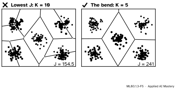
Wrong beside right. Of the values of \(K\) tried, \(K = 10\) has the lowest \(J\), and it cuts real blobs in half. The bend of the elbow, \(K = 5\), gives one cluster per blob.
“Pick the K with the lowest J.”
\(J\) always falls as \(K\) grows, so its minimum is wherever you stopped trying. Read the curve for a bend. If there is no clear bend, there may be no natural number of clusters at all; lesson ML03.10 treats the silhouette, the gap statistic and stability, which ask that question more carefully.
“KMeans already runs ten starts, so local minima are taken care of.”
That was true before scikit-learn 1.4. Now the default n_init="auto" runs k-means++ once. It is a good start, but in this lesson’s experiment 12 of 100 k-means++ seedings still ended in a poor local minimum. Set n_init yourself when it matters, and compare inertia_ between runs.
“k-means++ finds the best clustering.”
It is a randomised way to start. Its guarantee is on the expected \(J\) of the seeding, within a factor of \({8\,(\ln K + 2)}\) of the best, not a promise for any one run. Lloyd’s algorithm still stops at a local minimum.
Check yourself
Recall
1. In k-means++, with what probability is a point chosen as the next centre?
Show answer
Proportional to \(D(\vect{x})^2\), its squared distance to the nearest centre chosen so far: \(p_i = D(\vect{x}_i)^2 / \sum_j D(\vect{x}_j)^2\).
2. What does Arthur and Vassilvitskii’s theorem promise?
Show answer
That the expected \(J\) of the k-means++ seeding is at most \(8(\ln K + 2)\) times the lowest possible \(J\).
3. Why are several starts run, and which run is kept?
Show answer
Because each run can stop at a different local minimum. The run with the lowest \(J\) is kept.
4. What does scikit-learn’s KMeans do by default in version 1.9?
Show answer
It seeds with greedy k-means++ and, with n_init="auto", runs Lloyd’s algorithm once from that seed.
5. Why is the minimum of \(J\) over \(K\) no guide to the number of clusters?
Show answer
Because the best \(J\) falls every time \(K\) grows, reaching \(0\) with one cluster per point, so the minimum is always at the largest \(K\) tried.
Exercises
1.★ Points on a line at \(0, 1, 10, 11\). k-means++ chose \(0\) as the first centre. Find the probability that the second centre is \(10\) or \(11\).
Show solution
The squared distances to \(0\) are \(0, 1, 100, 121\), adding to \(222\). The probability is \({(100 + 121)/222} = 221/222 \approx 0.995\).
2.★★ One run of k-means reaches the best \(J\) with probability \(0.55\). How many independent runs are needed for the chance that none of them reaches it to fall below one in a thousand?
Show solution
All \(m\) runs fail with probability \(0.45^m\). We need \(0.45^m < 0.001\), so \(m \ln 0.45 < \ln 0.001\). Dividing by the negative number \(\ln 0.45 \approx -0.799\) flips the inequality: \(m > 6.908 / 0.799 \approx 8.65\). So \(m = 9\) runs: \({0.45^9} \approx 0.00076\), while \({0.45^8} \approx 0.0017\).
3.★★★ Prove that the best \(J\) with \(K + 1\) clusters is strictly lower than the best \(J\) with \(K\) clusters, as long as some cluster of the best \(K\)-clustering contains two points that are not equal.
Show solution
Take the best \(K\)-clustering and a cluster \(C\) with two unequal points. Its mean cannot equal both of them, so it contains a point \(\vect{x}\) with \(\vect{x} \ne \vect{\mu}_C\), whose term in \(J\) is \(\norm{\vect{x} - \vect{\mu}_C}^2 > 0\). Make \(\vect{x}\) a cluster of its own with centre \(\vect{x}\), and leave every other centre and assignment unchanged. The term of \(\vect{x}\) becomes \(0\) and no other term changes, so this \((K + 1)\)-clustering has a \(J\) strictly below \(J^*(K)\). The best \((K + 1)\)-clustering is at least as good, so \(J^*(K + 1) < J^*(K)\). (Re-centring \(C\) without \(\vect{x}\) would lower \(J\) further, but it is not needed for the proof.)
Summary card
Start spread out, keep the best of several runs, and read the elbow for a bend.
ML03.1.3-F1
The start decides the answer.
k-means++. Next centre with probability \(D(\vect{x})^2 / \sum D^2\).
Guarantee.\(\E[J] \le 8(\ln K + 2)\, J_{\text{opt}}\) for the seeding.
Several runs. Keep the lowest \(J\); scikit-learn’s default is one k-means++ run.
Choosing K.\(J\) always falls; look for the bend, not the minimum.
Cost. About \(n K d\) per round; mini-batches cut it to \(b K d\).
Sources and next steps
Sources. Each was opened and checked against this lesson on 15 November 2026.
David Arthur and Sergei Vassilvitskii, k-means++: The Advantages of Careful Seeding, Stanford University. Section 2.2 gives the seeding steps 1a to 1c with probability \(D(x)^2 / \sum D(x)^2\) (“\(D^2\) weighting”); Theorem 3.1 states \(\E[\phi] \le 8(\ln k + 2)\phi_{\text{OPT}}\); the introduction notes that \(\phi / \phi_{\text{OPT}}\) is unbounded for standard seeding.
scikit-learn developers, sklearn.cluster.KMeans, version 1.9.1. init="k-means++" implements “greedy k-means++”, which makes several trials at each sampling step; n_init="auto" gives 1 run for k-means++ and 10 for random starts, changed in version 1.4. The number of trials, \({2 + \lfloor \ln K \rfloor}\), is in the library’s source, _kmeans.py.
scikit-learn developers, User Guide, Section 2.3.2 K-means, version 1.9. Convergence may be to a local minimum, so the computation is often done several times; Mini Batch K-Means uses random mini-batches and gives results generally only slightly worse. The image comes from load_sample_image, shape (427, 640, 3).
Trevor Hastie, Robert Tibshirani and Jerome Friedman, The Elements of Statistical Learning, 2nd edition. Section 14.3.11 explains why \(W_K\) falls with \(K\) even on test data and reads the curve for a kink.