An embedding is judged by what it keeps. Measure trustworthiness and continuity from neighbour ranks, the share of nearest neighbours preserved, the Shepard diagram of distances and a k-NN classifier in the map, for PCA, Isomap, t-SNE and UMAP on 500 digits.
ML03.10.4L2 Intermediate25 minIn review (what this means)
The maths and code on this page are checked by automated tests on every change, but an independent reader has not signed it off yet. Spot a mistake or a confusing step? Tell us.
Explain the two kinds of neighbourhood error in a map, intruders and lost neighbours, and relate them to precision and recall.
Define trustworthiness and continuity by rank penalties, derive their normalising constant, and compute both by hand and from scratch.
Measure the share of nearest neighbours kept, draw and read a Shepard diagram, and use a k-NN classifier in the map as a downstream check.
Compare PCA, Isomap, t-SNE and UMAP on the same data, and explain why a picture with neat clusters proves nothing by itself.
The question
A t-SNE map of 500 handwritten digits shows ten neat islands; a PCA map of the same digits shows one smeared cloud. The t-SNE map looks better, but looking is not measuring. Which map keeps more of what is true about the data, and what exactly should “keep” mean?
From the last lesson
1. Which \(K\) does the gap statistic choose for the nine points, and why not the \(K\) with the largest gap?
Show answer
\({K} = {2}\). The gap is largest at \({K} = {3}\) (\({0.643}\)), but \({\mathrm{Gap}(2) = 0.416}\) is at least \({\mathrm{Gap}(3) - s_3} = {0.264}\), and the rule takes the smallest such \(K\).
2. Why is a stable clustering not proof of structure?
Show answer
Stability shows only that the answer is reproducible. If the best split of featureless data is unique, as for the uniform rectangle at \({K} = {2}\), it is found every time.
Intuition
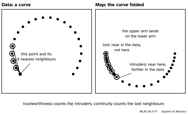
A map from many dimensions to two cannot keep every distance. So decide what matters. For exploring data the usual answer is neighbourhoods: points that are close in the data should be close in the map, and points close in the map should have been close in the data. Those are two different promises, and a map can break either one.
ML03.10.4-F1
A map that folds a curve. Around the black point, three map neighbours are intruders: the fold brings them down from farther up the curve, where they were only the 5th to 7th nearest. Three of its true neighbours are lost. Trustworthiness measures the first failure, continuity the second.
Venna and colleagues put this in the language of search. Treat the map as a search engine: ask for the neighbours of a point and see what comes back. Intruders are false positives, so they lower the precision; lost neighbours are misses, so they lower the recall.
Build it up
Step 1. Count the neighbours kept. For each point, take its \(k\) nearest neighbours in the data and its \(k\) nearest in the map, and count how many are in both. Averaged over points and divided by \(k\), this is the share of neighbours preserved. With both lists of length \(k\), precision and recall are this same number.
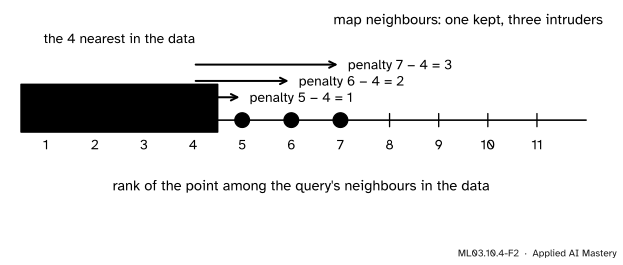
Step 2. Weigh each mistake. An intruder that was the data’s 5th neighbour, just outside the top 4, is a small mistake. One that was the 400th is a large one. So charge each intruder by how far down the data’s ranking it really sits: rank \(r\) costs \({r - k}\).
ML03.10.4-F2
The penalties of the folded curve’s black point, with \({k} = {4}\). Its map neighbours sit at ranks 1, 5, 6 and 7 in the data; each intruder costs its rank minus \(k\).
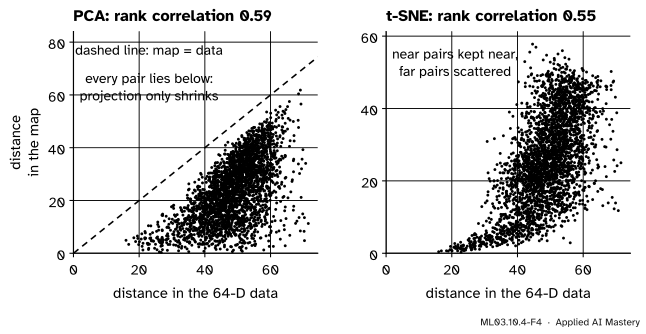
Step 3. Look at all distances. Plot, for every pair of points, the distance in the map against the distance in the data. This is a Shepard diagram. A perfect map puts every pair on one rising curve; its rank correlation summarises how faithfully the order of distances survives.
ML03.10.4-F4
Shepard diagrams of 3000 pairs of digits. PCA is an orthogonal projection, so no pair moves farther apart. t-SNE keeps near pairs near but scatters the far ones.
Step 4. Ask a downstream question. If the data carry labels, train a \(k\)-nearest-neighbour classifier on the map’s two coordinates and measure its cross-validated accuracy. A map that keeps classes apart scores high, a smeared one low. It tests usefulness for one task, not faithfulness.
The formal statement
NoteTrustworthiness and continuity (Venna and Kaski, 2001)
For point \(i\), let \({r(i, j)}\) be the rank of \(j\) among the neighbours of \(i\) in the data and \({\hat r(i, j)}\) its rank in the map, the nearest having rank 1. Let \(U_i^k\) hold the points among the \(k\) nearest of \(i\) in the map but not in the data (intruders), and \(V_i^k\) those among the \(k\) nearest in the data but not in the map (lost). With \({A = 2/(n k (2n - 3k - 1))}\),
Both equal 1 for a map that keeps every \(k\)-neighbourhood. Continuity is trustworthiness with the roles of data and map swapped.
Where \(A\) comes from. It scales the worst possible map to 0. The worst case for point \(i\) is that its \(k\) map neighbours are the \(k\) points farthest from it in the data, with ranks \({n - k}\) to \({n - 1}\). Their penalties are \({n - 2k}\) up to \({n - k - 1}\): \(k\) whole numbers in a row, whose average is the mean of the first and last,
Over all \(n\) points the worst total is \({\tfrac12\, n k (2n - 3k - 1)}\), and \(A\) is one over it. The argument needs the \(k\) farthest points to lie outside the \(k\) nearest, which holds when \({k < n/2}\); scikit-learn refuses larger \(k\).
Share preserved.\({Q(k)} = {\frac{1}{nk} \sum_i \abs{N_i^k \cap \hat N_i^k}}\), where \(N_i^k\) and \({\hat N_i^k}\) are the \(k\) nearest neighbours in the data and in the map. It ignores how wrong an intruder is, which \(T\) and \(C\) add.
Worked example
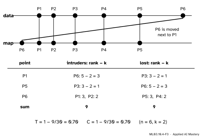
Six points on a line, at \(0\), \(1\), \(2.5\), \(4.5\), \(7\) and \(10\), called P1 to P6. The map is perfect except that P6 is drawn at \(-1.2\), next to P1. Take \({k} = {2}\).
Who changed. P2, P3 and P4 keep both neighbours. P1’s map neighbours are P2 and P6 instead of P2 and P3; P5’s are P4 and P3 instead of P4 and P6; P6’s are P1 and P2 instead of P5 and P4.
Intruders. For P1, P6 is the 5th nearest in the data (distances \({1, 2.5, 4.5, 7, 10}\)), so it costs \({5 - 2 = 3}\). For P5, P3 is 3rd in the data (after P4 at \(2.5\) and P6 at \(3\)), costing \(1\). For P6, P1 and P2 are 5th and 4th in the data, costing \({3 + 2 = 5}\). Total \(9\).
Lost neighbours. For P1, P3 is 3rd in the map (after P2 at \(1\) and P6 at \(1.2\)): cost \(1\). For P5, P6 is now 5th in the map: cost \(3\). For P6, P5 and P4 are 5th and 4th in the map: cost \({3 + 2 = 5}\). Total \(9\).
The scores.\({A} = {2/(6 \cdot 2 \cdot 5)} = {1/30}\), so \({T = 1 - 9/30 = 0.70}\) and \({C = 1 - 9/30 = 0.70}\).
ML03.10.4-F3
One misplaced point costs both scores: it brings intruders into two neighbourhoods and leaves its own true neighbours behind. Each penalty is a rank minus \(k\).
Code
Ranks, \(T\) and \(C\) from scratch, checked on the six points against scikit-learn, which computes continuity when the two arguments are swapped.
import numpy as npfrom sklearn.manifold import trustworthinessdef ranks(Z):"""R[i, j] = rank of j among the neighbours of i (the point itself has rank 0).""" D = ((Z[:, None, :] - Z[None, :, :]) **2).sum(-1) np.fill_diagonal(D, -1.0) order = np.argsort(D, axis=1, kind="stable") R = np.empty_like(order) R[np.arange(len(Z))[:, None], order] = np.arange(len(Z))return Rdef neighbourhood_scores(X, Y, k): n =len(X); RX, RY = ranks(X), ranks(Y) NX, NY = (RX >=1) & (RX <= k), (RY >=1) & (RY <= k) A =2/ (n * k * (2* n -3* k -1)) T =1- A * ((RX - k) * (NY &~NX)).sum() # intruders, charged by their data rank C =1- A * ((RY - k) * (NX &~NY)).sum() # lost neighbours, charged by their map rank Q = (NX & NY).sum() / (n * k) # share of neighbours keptreturn T, C, Qdata = np.array([[0], [1], [2.5], [4.5], [7], [10.0]])moved = data.copy(); moved[5] =-1.2T6, C6, Q6 = neighbourhood_scores(data, moved, 2)print(f"T = {T6:.2f}, C = {C6:.2f}, share kept = {Q6:.3f}")
T = 0.70, C = 0.70, share kept = 0.667
Now four maps of the 500 digits used in ML03.6. UMAP is the simplified version built in ML03.6.4, because the umap-learn library is not pinned for this course; with it installed, umap.UMAP(random_state=0).fit_transform(X) would take its place.
The simplified UMAP of ML03.6.4
from scipy.linalg import eighfrom scipy.optimize import curve_fitdef umap(X, k=15, min_dist=0.1, epochs=200, negatives=5, seed=0): d = np.linspace(0, 3, 300) target = np.where(d < min_dist, 1.0, np.exp(-(d - min_dist))) (a, b), _ = curve_fit(lambda d, a, b: 1/ (1+ a * d ** (2* b)), d, target)def find_sigma(ds): rho, lo, hi, s = ds[0], 0.0, np.inf, 1.0for _ inrange(64): total = np.exp(-np.maximum(ds - rho, 0) / s).sum()ifabs(total - np.log2(k)) <1e-5: break lo, hi = (lo, s) if total > np.log2(k) else (s, hi) s = (lo + hi) /2if hi < np.inf else2* sreturn s D = np.sqrt(((X[:, None] - X[None]) **2).sum(-1)); np.fill_diagonal(D, np.inf) idx = np.argsort(D, axis=1)[:, :k]; A = np.zeros(D.shape)for i inrange(len(X)): ds = D[i, idx[i]]; A[i, idx[i]] = np.exp(-np.maximum(ds - ds[0], 0) / find_sigma(ds)) W = A + A.T - A * A.T rng = np.random.default_rng(seed); deg = W.sum(1) Y = eigh(np.diag(deg) - W, np.diag(deg), subset_by_index=[1, 2])[1]; Y =10* Y / np.abs(Y).max() i, j = np.nonzero(np.triu(W)); p = W[i, j]for e inrange(epochs): step =1- e / epochs; take = rng.random(len(p)) < p; hi, hj = i[take], j[take] diff = Y[hi] - Y[hj]; s = (diff **2).sum(1) pull = np.clip(-2* a * b * s ** (b -1) / (1+ a * s ** b) * diff.T, -4, 4).T G = np.zeros_like(Y); np.add.at(G, hi, pull); np.add.at(G, hj, -pull) heads = np.repeat(hi, negatives); tails = rng.integers(0, len(Y), len(heads)) diff = Y[heads] - Y[tails]; s = (diff **2).sum(1) push =2* b / ((0.001+ s) * (1+ a * s ** b)) * (heads != tails) np.add.at(G, heads, np.clip(push * diff.T, -4, 4).T); Y = Y + step * Greturn Y
from scipy.spatial.distance import pdistfrom scipy.stats import spearmanrfrom sklearn.datasets import load_digitsfrom sklearn.decomposition import PCAfrom sklearn.manifold import TSNE, Isomapfrom sklearn.model_selection import cross_val_scorefrom sklearn.neighbors import KNeighborsClassifierX, labels = load_digits(return_X_y=True)pick = np.random.default_rng(0).choice(len(X), 500, replace=False)X, labels = X[pick], labels[pick]maps = {"PCA": PCA(2).fit_transform(X),"Isomap": Isomap(n_neighbors=10, n_components=2).fit_transform(X),"t-SNE": TSNE(2, perplexity=30, init="pca", random_state=0).fit_transform(X),"UMAP": umap(X)}knn = KNeighborsClassifier(5)dX = pdist(X)results = {}for name, Y in maps.items(): T, C, Q = neighbourhood_scores(X, Y, 10) acc = cross_val_score(knn, Y, labels, cv=5).mean() rho = spearmanr(dX, pdist(Y))[0] results[name] = (T, C, Q, acc, rho)print(f"{name:7s} T {T:.3f} C {C:.3f} kept {Q:.2f} 5-NN accuracy {acc:.3f} Shepard rho {rho:.2f}")print("5-NN accuracy in all 64 dimensions:", round(cross_val_score(knn, X, labels, cv=5).mean(), 3))
PCA     T 0.830  C 0.932  kept 0.24  5-NN accuracy 0.662  Shepard rho 0.59
Isomap  T 0.883  C 0.966  kept 0.37  5-NN accuracy 0.776  Shepard rho 0.56
t-SNE   T 0.983  C 0.975  kept 0.66  5-NN accuracy 0.954  Shepard rho 0.55
UMAP    T 0.978  C 0.973  kept 0.55  5-NN accuracy 0.964  Shepard rho 0.45
5-NN accuracy in all 64 dimensions: 0.966
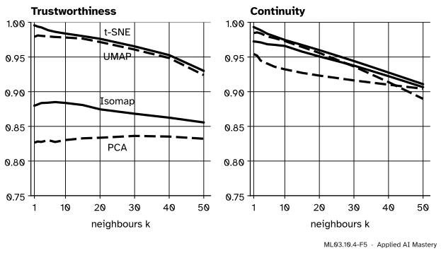
With \({k} = {10}\), PCA scores \({T = 0.830}\) and keeps only a quarter of each neighbourhood, and its 5-NN accuracy is about \(0.66\). t-SNE and UMAP keep more than half of each neighbourhood, their intruders come from close by (\({T \approx 0.98}\)), and their 5-NN accuracy, about \(0.95\) to \(0.96\), almost matches the \(0.966\) of all 64 pixels. But the Shepard rank correlation runs the other way: PCA keeps the order of all distances best (\({\rho = 0.59}\)), UMAP worst. t-SNE’s and UMAP’s values depend on their seeds, so they are checked with a tolerance.
ML03.10.4-F5
Trustworthiness and continuity for \({k} = {1}\) to \(50\). The neighbour-embedding maps lead on both at small \(k\). PCA and Isomap lose much more on trustworthiness than on continuity: their maps squash far points together.
Explore
The live t-SNE of ML03.6.3 runs on points you choose. Use its uniform noise preset at perplexity 2 and then 30, and ask of each picture the question of this lesson: would its clumps survive a check in the original data? The cluster scorecard of the last lesson gives that check for clusters.
Pitfalls
ML03.10.4-F6
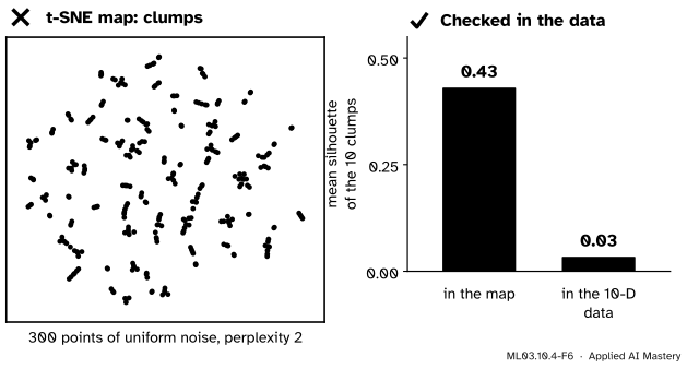
Wrong beside right. At perplexity 2, t-SNE draws uniform noise as tidy clumps, and ten clumps found in the map score a silhouette of \(0.44\) there. Measured in the original data, the same groups score \(0.04\): there is nothing to find.
“The t-SNE map shows clear clusters, so the data have clusters.”
A neighbour-embedding map is built to separate neighbourhoods, and at a small perplexity it separates noise into clumps (Wattenberg, Viégas and Johnson, section 4). Clusters seen in a map are a hypothesis. Test them in the original space, with the indices and the gap statistic of this module, and across settings and seeds (ML03.6.3).
“High trustworthiness means the whole picture is right.”
\(T\) and \(C\) look only at the \(k\) nearest neighbours. t-SNE has the highest trustworthiness here and still a lower Shepard correlation than PCA: the sizes of its islands and the gaps between them carry little meaning (Distill, sections 2 and 3). Choose the measure that matches the question: local neighbourhoods, global distances, or a downstream task.
“Report one number at one k.”
The ranking of maps can change with \(k\), and the values depend on \(n\) and on the distance used in the data. Show the curves over a range of \(k\), as in the figure above, and compare maps only on the same points with the same metric.
Check yourself
Recall
1. What is an intruder, and which measure does it lower?
Show answer
A point among the \(k\) nearest neighbours of \(i\) in the map that is not among its \(k\) nearest in the data. It lowers trustworthiness.
2. How is an intruder penalised in \({T(k)}\)?
Show answer
By \({r(i, j) - k}\), how far beyond the \(k\) nearest it sits in the data’s ranking.
3. What does the constant \({2/(nk(2n - 3k - 1))}\) do?
Show answer
It divides by the largest possible total penalty, so that the worst map scores 0 and a perfect one 1.
4. What does a Shepard diagram plot?
Show answer
For every pair of points (or a sample of pairs), the distance in the map against the distance in the data.
5. Why does a high k-NN accuracy in the map not prove the map is faithful?
Show answer
It only shows that the map keeps the classes apart. A map can separate classes while distorting distances and neighbourhoods within and between them, and it says nothing about data without labels.
Exercises
1.★ With \({n} = {100}\) points and \({k} = {5}\), what is the normalising constant \(A\), and what is \(T\) if the intruders’ penalties add to \(970\)?
2.★★ In the six-point example, move P6 back to \(10\) but draw P3 at \(8.5\) instead of \(2.5\). Find P2’s intruders and their penalties with \({k} = {2}\).
Show solution
The map positions are \({0, 1, 8.5, 4.5, 7, 10}\). From P2 at \(1\): P1 is \(1\) away, P4 \(3.5\), P5 \(6\), P3 \(7.5\), P6 \(9\), so its map neighbours are P1 and P4. In the data its neighbours are P1 (distance 1) and P3 (1.5); P4 is at distance 3.5, rank 3. So P4 is an intruder with penalty \({3 - 2 = 1}\), and P3 is lost, now at map rank 4, costing \({4 - 2 = 2}\) in continuity.
3.★★★ Show that for an orthogonal projection onto principal directions, every map distance is at most the data distance, and explain why that makes PCA’s Shepard diagram lie under the diagonal.
Show solution
The map is \({\vect{y}} = {\mat{Q}_q\T(\vect{x} - \bar{\vect{x}})}\) with orthonormal columns in \(\mat{Q}_q\). For two points, \({\vect{y}_i - \vect{y}_j} = {\mat{Q}_q\T \vect{v}}\) with \({\vect{v}} = {\vect{x}_i - \vect{x}_j}\). Complete \(\mat{Q}_q\) to an orthonormal basis \(\mat{Q}\) of \(\R^d\). Then \({\norm{\vect{v}}^2} = {\norm{\mat{Q}\T\vect{v}}^2}\) is the sum of the squares of all \(d\) coordinates of \(\vect{v}\) in that basis, and \({\norm{\mat{Q}_q\T \vect{v}}^2}\) keeps only the first \(q\) of those squares. Dropping non-negative terms cannot increase a sum, so \({\norm{\vect{y}_i - \vect{y}_j}} \le {\norm{\vect{x}_i - \vect{x}_j}}\), and every pair lies on or below the line where map distance equals data distance.
Summary card
An embedding is judged by what it keeps: neighbours, distances, or usefulness.
Shepard diagram. Map distance against data distance for every pair.
Digits. t-SNE and UMAP: \({T} \approx {0.98}\), 5-NN about \(0.95\); PCA: \({T} = {0.83}\), but the best \(\rho\).
Sources and next steps
Sources. Each was opened and checked against this lesson on 15 November 2026.
Samuel Kaski, Janne Nikkilä, Merja Oja, Jarkko Venna, Petri Törönen and Eero Castrén, Trustworthiness and metrics in visualizing similarity of gene expression, BMC Bioinformatics 4 (2003), article 48. The Methods subsection on measuring trustworthiness defines it from the samples \({U_k(x_i)}\) that are neighbours on the display but not in the original space, ranked by \({r(x_i, x_j)}\), with the scale \({A(k)} = {2/(Nk(2N - 3k - 1))}\); the preservation of the original neighbourhoods uses \({V_k(x_i)}\) and display ranks \({\hat r}\) in the same way.
Jarkko Venna, Jaakko Peltonen, Kristian Nybo, Helena Aidos and Samuel Kaski, Information Retrieval Perspective to Nonlinear Dimensionality Reduction for Data Visualization, Journal of Machine Learning Research 11 (2010), 451 to 490. Section 2.1.2 and Figure 1 read the errors of a visualisation as misses and false positives, that is, recall and precision, and Section 2.1.3 notes that the two are equal when as many points are retrieved as are relevant; Section 4.3.1 uses trustworthiness and continuity and a 5-nearest-neighbour classifier in the display as measures.
scikit-learn developers, sklearn.manifold.trustworthiness, version 1.9. The formula with ranks \({r(i, j)}\) in the input space, the requirement that n_neighbors be below n_samples / 2, and the reference to Venna and Kaski (2001).
Martin Wattenberg, Fernanda Viégas and Ian Johnson, How to Use t-SNE Effectively, Distill (2016). Sections 2, 3 and 4: cluster sizes in a t-SNE plot mean nothing, distances between clusters might not mean anything, and random noise does not always look random.
Next. Learned embeddings, such as those of a neural network, are probed and evaluated in DL08.7 (transfer and probing) and DL08.8 (evaluating embeddings and retrieval).