UMAP builds a weighted nearest-neighbour graph with a local scale at every point, joins the two directions of each edge by a fuzzy union, and lays the graph out by stochastic gradient descent on a cross-entropy with negative sampling. Build a simplified UMAP and compare it with t-SNE.
ML03.6.4L2 Intermediate30 minIn review (what this means)
The maths and code on this page are checked by automated tests on every change, but an independent reader has not signed it off yet. Spot a mistake or a confusing step? Tell us.
Compute UMAP’s edge weights for a point: rho_i, the sigma_i that makes the weights add up to log2 k, and the fuzzy union p + p’ - p p’.
Explain the map’s curve 1/(1 + a d^(2b)), how min_dist sets a and b, and derive the attractive and repulsive gradients of the cross-entropy.
Build a simplified UMAP from scratch with negative sampling on 500 digits and compare it with t-SNE as n_neighbors and min_dist change.
Place new points on an existing UMAP map, which t-SNE cannot do.
The question
t-SNE draws beautiful maps, but each run must see all the data at once, every iteration of the exact method touches every pair of points, and a new image cannot be added to a finished map. UMAP, published in 2018, draws maps of the same kind and is widely used in its place. What does it keep from t-SNE, and what does it change to be fast and to take new points?
From the last lesson
1. What does early exaggeration do?
Show answer
It multiplies every \(p_{ij}\) by a factor for the first iterations, pulling neighbours into tight, well-separated clumps that can move past each other.
2. Name two things a t-SNE map cannot be trusted to show.
Show answer
The relative sizes of clusters and the distances between well-separated clusters (and clumps at low perplexity can be pure noise).
Intuition
UMAP goes back to the graph of the first lesson. Each point is joined to its \(k\) nearest neighbours, and each edge gets a weight between 0 and 1, read as the chance that the edge is really there. Then a map is drawn in which joined points sit close and unjoined points sit apart, by tugging on one edge at a time.
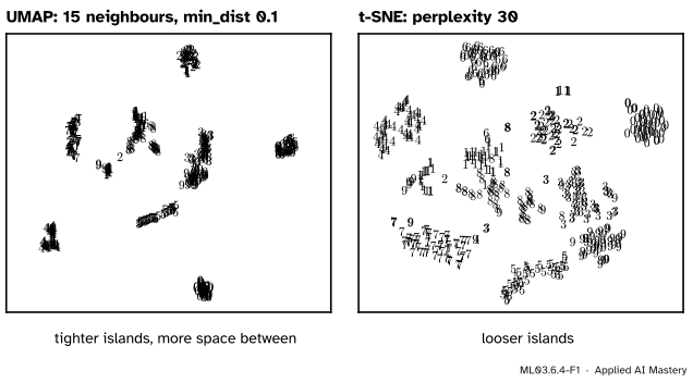
ML03.6.4-F1
The same 500 digits, laid out by a simplified UMAP built in this lesson (left) and by t-SNE (right). UMAP packs each group more tightly and leaves more space between groups.
Two differences from t-SNE drive everything. The weights are not normalised to add up to 1 over all pairs, so each edge can be treated on its own, and a sample of edges is enough for each update. And the cost charges for unjoined points drawn close as well as for joined points drawn apart.
Build it up
Step 1. Neighbours. For each point \(i\), find its \(k\) nearest neighbours (n_neighbors, 15 by default) and their distances \(d_{i1} \le \dots \le d_{ik}\).
Step 2. A local scale. Let \({\rho_i = d_{i1}}\), the distance to the nearest neighbour, and give each edge the weight
The nearest neighbour always gets weight 1, so no point is left alone however sparse its region. \(\cparam{\sigma_i}\) is set by binary search so that
\[
\sum_{j=1}^{k} v_{j|i} = \log_2 k ,
\]
the same idea as t-SNE’s perplexity: every point gets the same total amount of neighbourhood.
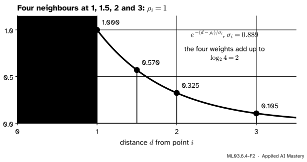
ML03.6.4-F2
Four neighbours at 1, 1.5, 2 and 3. The weight is 1 up to the nearest neighbour and then decays; \({\sigma_i = 0.889}\) makes the four weights add up to \({\log_2 4 = 2}\).
Step 3. One weight per edge.\(v_{j|i}\) and \(v_{i|j}\) usually differ. Reading each as the chance that a directed edge exists, the chance that at least one exists is the fuzzy union
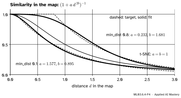
With \({a = b = 1}\) this is t-SNE’s Student t, unnormalised. UMAP fits \(a\) and \(b\) so that \(\Phi\) is close to a target that is 1 up to the distance min_dist and then decays like \({e^{-(d - \text{min\_dist})}}\): for the default \({\text{min\_dist} = 0.1}\), \({a = 1.577}\) and \({b = 0.895}\).
ML03.6.4-F4
The map’s similarity curve for two values of min_dist. A larger min_dist keeps the similarity near 1 out to a larger distance, so points need not crowd together to count as close.
The formal statement
NoteThe UMAP cost: cross-entropy over all pairs
With \({\Phi_{ij} = \Phi(\norm{\vect{y}_i - \vect{y}_j})}\),
The first term attracts the ends of every edge; the second repels every pair that is not a sure edge.
For one pair, \(\closs{C}\) is smallest when \({\Phi_{ij} = p_{ij}}\): setting the derivative \({-p/\Phi + (1 - p)/(1 - \Phi)}\) to zero gives \({\Phi = p}\). So each pair has a preferred distance in the map, and the layout balances all of them.
The gradients. Write \({s = \norm{\vect{y}_i - \vect{y}_j}^2}\), so \({\Phi = (1 + a s^b)^{-1}}\) and \({\partial s/\partial\vect{y}_i = 2(\vect{y}_i - \vect{y}_j)}\). For the attractive term, \({-\log\Phi = \log(1 + a s^b)}\), and
with \({\vect{u} = \vect{y}_i - \vect{y}_j}\). The second line puts both fractions over \({s(1 + as^b)}\): the numerator \({2ab\,s^b - 2b(1 + as^b)}\) is \({-2b}\). A descent step moves \(\vect{y}_i\) against the gradient: the first term pulls it towards \(\vect{y}_j\), the second pushes it away. In code, \(s\) in the repulsion gets a small \({\epsilon = 0.001}\) added, so that two points on top of each other do not divide by zero.
Stochastic gradient descent with negative sampling. The repulsive sum has a term for every pair, \({n^2/2}\) of them, but most have \({p_{ij} \approx 0}\) and only matter as “keep apart”. So each epoch goes through the edges, takes an edge with probability \(p_{ij}\), applies the attractive step to both ends, and then applies the repulsive step between \(\vect{y}_i\) and a few points drawn at random (5 by default), treated as non-edges. The step size falls linearly from 1 to 0 over the epochs. The work per epoch grows with the number of edges, about \(nk\), not with \(n^2\). The start is the Laplacian eigenmap of the graph, from the first lesson.
Worked example
The weights of one point, one edge, and where the edge wants to rest. Point \(i\) has \(k = 4\) neighbours at distances 1, 1.5, 2 and 3.
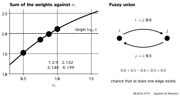
Try \({\sigma = 1}\): \({1 + 0.607 + 0.368 + 0.135 = 2.11}\), too much, so halve: \({\sigma = 0.5}\) gives \({1 + 0.368 + 0.135 + 0.018 = 1.52}\), too little. Bisect: 0.75 gives 1.85, 0.875 gives 1.99, 0.9375 gives 2.05. The search settles at \({\sigma_i = 0.889}\), with weights 1, 0.570, 0.325 and 0.105.
Fuzzy union. Say \(i\) gives its neighbour \(j\) the weight 0.6 and \(j\) gives \(i\) the weight 0.5. Then \({p_{ij} = 0.6 + 0.5 - 0.6 \times 0.5 = 0.8}\).
ML03.6.4-F3
Left: binary search for \(\sigma_i\): the sum of the weights rises with \(\sigma_i\), and the search closes in on 2. Right: two directed weights become one undirected weight.
Where the edge rests. With \({a = 1.577}\) and \({b = 0.895}\), the edge is happiest where \({\Phi(d) = 0.8}\):
At \({d = 1}\), \({\Phi = 1/2.577 = 0.388}\) and the edge’s cost is \({-[0.8\ln 0.388 + 0.2\ln 0.612] = 0.856}\); at \({d = 0.357}\) it falls to its least, 0.500. The two coefficients of the gradient at \({d = 1}\) are \({0.8 \times 2ab/(1 + a) = 0.876}\) (pull) and \({0.2 \times 2b/(1 + a) = 0.139}\) (push), so the edge pulls its ends together until they are 0.357 apart.
Code
A simplified UMAP: exact nearest neighbours, the weights of Step 2, the fuzzy union, \(a\) and \(b\) fitted with scipy.optimize.curve_fit, an eigenmap start, and epochs in which every edge drawn with probability \(p_{ij}\) pulls its two ends together and pushes its first end away from 5 random points. For speed, each epoch applies all its sampled updates at once.
import numpy as npfrom scipy.linalg import eighfrom scipy.optimize import curve_fitdef find_ab(min_dist, spread=1.0): d = np.linspace(0, 3* spread, 300) target = np.where(d < min_dist, 1.0, np.exp(-(d - min_dist) / spread)) (a, b), _ = curve_fit(lambda d, a, b: 1/ (1+ a * d ** (2* b)), d, target)return a, bdef find_sigma(dists, k): rho, lo, hi, s = dists[0], 0.0, np.inf, 1.0for _ inrange(64): total = np.exp(-np.maximum(dists - rho, 0) / s).sum()ifabs(total - np.log2(k)) <1e-5: break lo, hi = (lo, s) if total > np.log2(k) else (s, hi) s = (lo + hi) /2if hi < np.inf else2* sreturn sdef fuzzy_graph(X, k): D = np.sqrt(((X[:, None] - X[None]) **2).sum(-1)); np.fill_diagonal(D, np.inf) idx = np.argsort(D, axis=1)[:, :k] A = np.zeros(D.shape)for i inrange(len(X)): d = D[i, idx[i]] A[i, idx[i]] = np.exp(-np.maximum(d - d[0], 0) / find_sigma(d, k))return A + A.T - A * A.T # fuzzy uniondef umap(X, k=15, min_dist=0.1, epochs=200, negatives=5, seed=0): rng = np.random.default_rng(seed) a, b = find_ab(min_dist) W = fuzzy_graph(X, k) deg = W.sum(1) Y = eigh(np.diag(deg) - W, np.diag(deg), subset_by_index=[1, 2])[1] # eigenmap start Y =10* Y / np.abs(Y).max() i, j = np.nonzero(np.triu(W)); p = W[i, j]for e inrange(epochs): step =1- e / epochs take = rng.random(len(p)) < p # sample each edge with probability p_ij hi, hj = i[take], j[take] diff = Y[hi] - Y[hj]; s = np.maximum((diff **2).sum(1), 1e-12) # s^(b-1) needs s > 0 pull = np.clip(-2* a * b * s ** (b -1) / (1+ a * s ** b) * diff.T, -4, 4).T G = np.zeros_like(Y); np.add.at(G, hi, pull); np.add.at(G, hj, -pull) heads = np.repeat(hi, negatives); tails = rng.integers(0, len(Y), len(heads)) diff = Y[heads] - Y[tails]; s = (diff **2).sum(1) push =2* b / ((0.001+ s) * (1+ a * s ** b)) * (heads != tails) np.add.at(G, heads, np.clip(push * diff.T, -4, 4).T) Y = Y + step * Greturn Y, Wa, b = find_ab(0.1)sigma_i = find_sigma(np.array([1.0, 1.5, 2.0, 3.0]), 4)print(f"a = {a:.3f}, b = {b:.3f} sigma_i = {sigma_i:.3f} Phi(1) = {1/ (1+ a):.3f}")
a = 1.577, b = 0.895 sigma_i = 0.889 Phi(1) = 0.388
Now 500 digits, judged as before by a 5-nearest-neighbour classifier in the map, beside t-SNE, and with two other settings: how tightly do the islands pack (the median distance from a point to its nearest neighbour in the map, relative to the map’s size)?
UMAP k=15, min_dist 0.1    5-NN accuracy 0.964   nearest-neighbour gap 0.012
UMAP k=15, min_dist 0.8    5-NN accuracy 0.948   nearest-neighbour gap 0.035
UMAP k=50, min_dist 0.1    5-NN accuracy 0.952   nearest-neighbour gap 0.019
t-SNE perplexity 30        5-NN accuracy 0.954   nearest-neighbour gap 0.031
All four keep the digit groups (accuracy near 0.95). A larger min_dist spreads the points out, as its curve promised, and UMAP with the default packs points more tightly than t-SNE.
New points. Fit on 400 digits, then place each of the other 100 at the weighted mean of the map positions of its 15 nearest training digits, with the weights of Step 2: the first step of umap-learn’s transform, which then refines the position with a few epochs of the same descent.
train, test = np.arange(400), np.arange(400, 500)Y_train, _ = umap(X[train])D = np.sqrt(((X[test][:, None] - X[train][None]) **2).sum(-1))idx = np.argsort(D, axis=1)[:, :15]Y_test = np.zeros((len(test), 2))for r inrange(len(test)): d = D[r, idx[r]] w = np.exp(-np.maximum(d - d[0], 0) / find_sigma(d, 15)) Y_test[r] = w @ Y_train[idx[r]] / w.sum()placed = KNeighborsClassifier(5).fit(Y_train, labels[train]).score(Y_test, labels[test])print("new digits placed on the old map, 5-NN accuracy:", placed)
new digits placed on the old map, 5-NN accuracy: 0.95
With umap-learn, which is not pinned for this course, the same work is a few lines (not run here):
import umap # pip install umap-learnreducer = umap.UMAP(n_neighbors=15, min_dist=0.1, random_state=0)Y_train = reducer.fit_transform(X_train) # learn the mapY_test = reducer.transform(X_test) # place new points on it
Explore
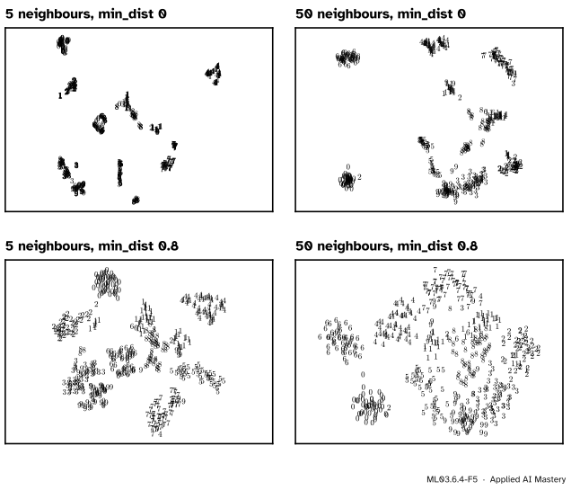
This module’s interactive, live t-SNE, lives in lesson 3. Its uniform-noise preset at low perplexity shows the same false structure that a small n_neighbors gives UMAP below.
ML03.6.4-F5
Two settings, four maps. Fewer neighbours (left) favours fine local structure and breaks groups up; more (right) favours the large picture. A larger min_dist (bottom) spreads points out inside every group.
Pitfalls
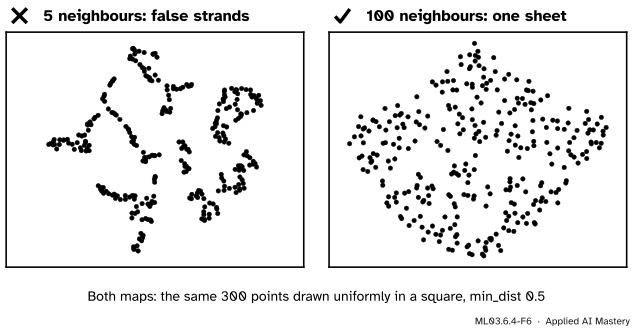
ML03.6.4-F6
Wrong beside right, both with min_dist 0.5. With 5 neighbours UMAP reads the random gaps of uniform noise as structure and draws strands; with 100 it draws one rough sheet.
“UMAP’s islands are real clusters.”
With a small n_neighbors, UMAP takes the chance gaps of random sampling for fine structure; its authors warn that low values can produce spurious structure. As with t-SNE, check a structure across settings and seeds before believing it, and test it with ML03.10.
“min_dist is a distance in the data.”
It lives in the map. It only shapes the curve \(\Phi\): how close two points must be drawn to count as neighbours. UMAP’s authors call it an essentially aesthetic parameter; a large value spreads points out (the nearest-neighbour gap above more than doubles from 0.1 to 0.8) without changing the graph.
“UMAP’s map distances can be read like PCA’s.”
Like t-SNE, UMAP keeps neighbourhoods. Sizes of groups and distances between them depend on n_neighbors, min_dist and the start; measure such things in the data.
Check yourself
Recall
1. How are \(\rho_i\) and \(\sigma_i\) chosen?
Show answer
\(\rho_i\) is the distance to \(i\)’s nearest neighbour; \(\sigma_i\) is found by binary search so that the \(k\) weights \({v_{j|i} = e^{-\max(0,\, d_{ij} - \rho_i)/\sigma_i}}\) add up to \({\log_2 k}\).
2. What is the fuzzy union of two directed weights?
Show answer
\({p_{ij} = v_{j|i} + v_{i|j} - v_{j|i}v_{i|j}}\): the chance that at least one of the two edges exists.
3. What does min_dist change?
Show answer
The curve \({\Phi(d) = (1 + a d^{2b})^{-1}}\) in the map: \(a\) and \(b\) are fitted to a target that is 1 up to min_dist, so a larger value lets close points sit further apart.
4. For a single pair, at what map distance is the cross-entropy smallest?
Show answer
Where \({\Phi(d) = p_{ij}}\).
5. What is negative sampling, and why is it needed?
Show answer
Instead of summing the repulsive term over all \({n^2/2}\) pairs, each sampled edge’s first end is pushed away from a few random points treated as non-edges. It makes an epoch cost about \(nk\) instead of \(n^2\).
Exercises
1.★ Point \(i\) has \(k = 2\) neighbours at distances 2 and 3. Find \(\rho_i\) and \(\sigma_i\).
Show solution
\({\rho_i = 2}\). The weights are 1 and \({e^{-1/\sigma}}\), and they must add up to \({\log_2 2 = 1}\). That needs \({e^{-1/\sigma} = 0}\), so \({\sigma_i \to 0}\): with two neighbours, \(i\) keeps only its nearest. (The binary search stops at a tiny \(\sigma_i\).) With \(k = 2\) the graph is almost a nearest-neighbour graph, one reason the default is 15.
2.★★ Show that for \({a = b = 1}\) the attractive coefficient \({2ab\,s^{b-1}/(1 + as^b)}\) is t-SNE’s \({w_{ij} = (1 + s)^{-1}}\) up to a factor, and say what is missing compared with t-SNE’s gradient.
Show solution
With \({a = b = 1}\), \({2ab\,s^{b-1}/(1 + as^b)} = {2/(1 + s)} = {2w_{ij}}\). t-SNE’s gradient is \({4(p_{ij} - q_{ij})w_{ij}(\vect{y}_i - \vect{y}_j)}\): its repulsion comes through \(q_{ij}\), which is normalised over all pairs, so every pair repels every other. UMAP has no normalisation; its repulsion is the separate term \({(1 - p_{ij})\,2b/(s(1 + as^b))}\), which can be estimated from a few sampled pairs.
3.★★★ For one pair with weight \(p\), prove that the cross-entropy \({-p\log\Phi - (1 - p)\log(1 - \Phi)}\) is smallest at \({\Phi = p}\), and find the resting distance for \({p = 0.5}\) with the default \(a\) and \(b\).
Show solution
As a function of \(\Phi\) in \({(0, 1)}\), the derivative is \({-p/\Phi + (1 - p)/(1 - \Phi)}\), which is negative for \({\Phi < p}\) and positive for \({\Phi > p}\), so the minimum is at \({\Phi = p}\). For \({p = 0.5}\): \({1 + a d^{2b} = 2}\), so \({d^{2b} = 1/a = 0.634}\) and \({d = 0.634^{1/1.790} = 0.775}\). A weaker edge rests further apart than the 0.357 of \({p = 0.8}\).
Summary card
A fuzzy neighbour graph, laid out one sampled edge at a time.
Map.\({\Phi(d) = (1 + a d^{2b})^{-1}}\), with \(a\), \(b\) fitted from min_dist.
Cost. Cross-entropy: attraction on edges, repulsion on non-edges, by negative sampling.
Unlike t-SNE. Cost per epoch about \(nk\); transform places new points.
Sources and next steps
Sources. Each was opened and checked against this lesson on 15 November 2026.
Leland McInnes, John Healy and James Melville, UMAP: Uniform Manifold Approximation and Projection for Dimension Reduction, arXiv:1802.03426, version 3. Section 3.1 defines \(\rho_i\), \(\sigma_i\) with the sum over the \(k\) neighbours equal to \({\log_2 k}\), the weights \({\exp(-\max(0, d - \rho_i)/\sigma_i)}\) and the symmetrisation \({B = A + A\T - A \circ A\T}\). Section 3.2 gives the attractive and repulsive forces (with \({\epsilon = 0.001}\)), the spectral start and the cross-entropy. Section 4.1 gives edge sampling with probability \(\mu(a)\), negative sampling, the curve \({\Phi = (1 + a\norm{x - y}^{2b})^{-1}}\) fitted to the target set by min-dist (Definition 11), and the step size \({1 - e/n_{\text{epochs}}}\) (Algorithm 5); Section 4.3 notes that low values of \(n\) can produce spurious structure and calls min-dist an essentially aesthetic parameter.
umap-learn documentation, Basic UMAP Parameters: n_neighbors (default 15) balances local against global structure; min_dist (default 0.1) controls how tightly points may be packed. Transforming New Data with UMAP: fit on training data, then transform on test data.
umap-learn source, umap/umap_.py: defaults n_neighbors=15, min_dist=0.1 and negative_sample_rate=5; find_ab_params fits \(a\) and \(b\) with curve_fit to the target used here; smooth_knn_dist aims at \({\log_2 k}\) with the point itself counted among the \(k\) neighbours; transform starts each new point at the weighted average of its neighbours’ positions (init_graph_transform) and then runs a few epochs.
Next. Module ML03.7, Matrix factorisation and topic models, turns from maps to factors; lesson ML03.10.4 measures how well an embedding keeps neighbourhoods.