Rotate a cloud onto its principal axes and divide by the spreads, and its covariance becomes the identity. Compare PCA and ZCA whitening, find the scores from a small n by n matrix when features outnumber examples, and recover PCA from a table of distances alone by classical MDS.
ML03.5.2L2 Intermediate25 minIn review (what this means)
The maths and code on this page are checked by automated tests on every change, but an independent reader has not signed it off yet. Spot a mistake or a confusing step? Tell us.
Whiten a data set by rotating onto its principal axes and dividing by the standard deviations, and check that the covariance becomes the identity.
Contrast PCA whitening with ZCA whitening, compute both for the four points, and match PCA(whiten=True).
Derive that the eigenvectors of the n by n matrix X_c X_c-transpose give the PCA scores, and use it when d exceeds n.
Derive that double centring a matrix of squared distances recovers X_c X_c-transpose, and run classical MDS from scratch and with ClassicalMDS.
The question
Many methods quietly assume that the features are uncorrelated and equally spread: k-means measures round distances, and the scikit-learn guide names RBF-kernel SVMs too. Real features are neither. Can we reshape a cloud so that it is perfectly round? And when all we have is a table of distances between items, with no coordinates at all, can PCA still be run?
From the last lesson
1. What is PCA’s mean squared reconstruction error, dividing by \(n - 1\), with \(q\) directions kept?
Show answer
The sum of the dropped eigenvalues, \({\lambda_{q+1} + \cdots + \lambda_d}\).
2. What is the covariance of the codes \({\vect{y} = \mat{Q}_q\T(\vect{x} - \bar{\vect{x}})}\)?
Show answer
The diagonal matrix of \({\lambda_1, \dots, \lambda_q}\): the codes are uncorrelated and code \(j\) has variance \(\lambda_j\).
Intuition
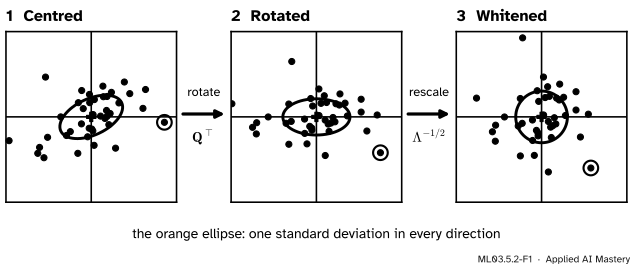
The second recall answer is the whole idea. PCA’s codes are already uncorrelated; they only differ in spread. Divide each code by its standard deviation and every direction has spread 1. That is whitening: two moves, a turn and a stretch.
ML03.5.2-F1
Whitening. Turning the cloud onto its principal axes removes the correlation; dividing each axis by its standard deviation makes every spread 1. The ellipse of one standard deviation becomes the unit circle.
After whitening no direction is special: the variance along every unit direction is 1. Algorithms that measure plain Euclidean distance then weigh every direction of the original data by how unusual a step along it is, not by its units.
Build it up
Step 1. Rotate. The scores \({\vect{y} = \mat{Q}\T(\vect{x} - \bar{\vect{x}})}\) have covariance \({\mat{Q}\T\mat{C}\mat{Q} = \mat{\Lambda}}\), the diagonal matrix of eigenvalues (ML03.5.1, exercise 3).
Step 2. Rescale. Divide score \(j\) by \(\sqrt{\lambda_j}\), that is multiply by \({\mat{\Lambda}^{-1/2}}\). A diagonal scaling multiplies the covariance on both sides, so the new covariance is \({\mat{\Lambda}^{-1/2}\mat{\Lambda}\mat{\Lambda}^{-1/2} = \mat{I}}\). Together,
This is PCA whitening, and it is what PCA(whiten=True) returns.
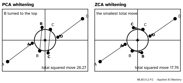
Step 3. Rotate back, if you like. Any rotation of a round cloud is still round, so turning \(\vect{z}\) back with \(\mat{Q}\) keeps the covariance at \(\mat{I}\). The result is ZCA whitening (zero-phase component analysis):
the inverse square root of \(\mat{C}\) (M03.3.3). Whitened data are therefore far from unique: Kessy, Lewin and Strimmer call this the rotational freedom of whitening. ZCA is the choice that keeps the data in their original axes, and it moves the points less than any other whitening.
ML03.5.2-F2
The four points whitened two ways. Both results are round, with covariance \(\mat{I}\); ZCA keeps each point closest to where it was, so images whitened by ZCA still look like images.
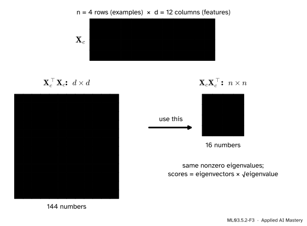
Step 4. More features than examples. Whitening, like PCA, needs the eigenvectors of the \({d \times d}\) matrix \({\mat{X}_c\T\mat{X}_c}\). For 300 photographs of a million pixels each, that is a million by a million. But 300 points span at most 299 directions, and there is a short cut.
ML03.5.2-F3
When \(d\) is larger than \(n\), work with the small \({n \times n}\) Gram matrix instead of the large \({d \times d}\) one.
Let \({\mat{X}_c\mat{X}_c\T\vect{u} = \mu\vect{u}}\) with \(\vect{u}\) a unit vector and \({\mu > 0}\). Multiply on the left by \(\mat{X}_c\T\):
So \({\mat{X}_c\T\vect{u}}\) is an eigenvector of the big matrix with the same eigenvalue \(\mu\). Its squared length is \({\vect{u}\T\mat{X}_c\mat{X}_c\T\vect{u} = \mu}\), so the unit principal direction is \({\vect{q} = \mat{X}_c\T\vect{u}/\sqrt{\mu}}\), and the scores are
The scores come straight from the small matrix: eigenvector times the square root of its eigenvalue. The variance along \(\vect{q}\) is \({\mu/(n - 1)}\). This is Bishop’s Section 12.1.4.
The formal statement
The small matrix \({\mat{B} = \mat{X}_c\mat{X}_c\T}\) holds the dot products of the centred points, \({b_{ij} = \vect{c}_i \cdot \vect{c}_j}\). The remarkable fact is that it can be rebuilt from distances alone.
NoteDouble centring
Let \({\mat{D}^{(2)}}\) hold the squared distances \({\norm{\vect{x}_i - \vect{x}_j}^2}\), and let \({\mat{J} = \mat{I} - \tfrac1n\vect{1}\vect{1}\T}\), the centring matrix. Then
Derivation. Put the origin anywhere and let \({\mat{G} = \mat{X}\mat{X}\T}\), with diagonal entries \({g_i = \norm{\vect{x}_i}^2}\). Expanding a squared distance,
so \({\mat{D}^{(2)} = \vect{g}\vect{1}\T + \vect{1}\vect{g}\T - 2\mat{G}}\). Now use two facts about \(\mat{J}\). First, \({\mat{J}\vect{1} = \vect{0}}\) and \({\vect{1}\T\mat{J} = \vect{0}\T}\), because \(\mat{J}\) subtracts the mean and a constant vector has nothing left. So
Entry by entry, double centring reads \({b_{ij} = -\tfrac12\,(D^{(2)}_{ij} - r_i - r_j + \bar{r})}\), where \(r_i\) is the mean of row \(i\) of \({\mat{D}^{(2)}}\) and \(\bar{r}\) the mean of all its entries.
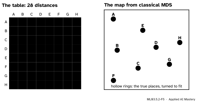
Classical MDS (multidimensional scaling) follows in one line. Take the top \(q\) eigenpairs \({(\mu_j, \vect{u}_j)}\) of \(\mat{B}\) and give point \(i\) the coordinates \({(\sqrt{\mu_1}\,u_{i1}, \dots, \sqrt{\mu_q}\,u_{iq})}\). By Step 4 these are exactly the PCA scores, up to the sign of each column. Points are placed from their distances, and nothing else.
ML03.5.2-F5
Classical MDS rebuilds the eight towns from their 28 distances. The map is the true layout up to a turn and a mirror image, which distances cannot see.
ML03.6.1 feeds classical MDS with distances measured along a neighbourhood graph instead of straight lines; that is Isomap.
Worked example
Whitening the four points. From M03.6, the four centred points are \({(-3.5, -2)}\), \({(-0.5, -1)}\), \({(0.5, 1)}\) and \({(3.5, 2)}\), with
Rotate. With \({\vect{q}_1 \approx (0.851, 0.526)}\) and \({\vect{q}_2 \approx (0.526, -0.851)}\), the first point has scores \({-4.03}\) and \({0.526 \times (-3.5) + (-0.851)(-2)} \approx -0.14\).
Rescale. Divide by \({\sqrt{11.42} \approx 3.380}\) and \({\sqrt{0.243} \approx 0.493}\): the first point becomes \({(-1.19, -0.28)}\). In each whitened column the squares add up to 3, so with \({n - 1 = 3}\) each variance is 1, and the cross-products cancel in pairs.
ZCA. Here \({\mat{C}^{-1/2}}\) has a tidy form. Check that the matrix
For the first entry of \({\mat{C}\mat{M}^2}\), \({(25 \times 2 - 15 \times 3)/5 = 1}\); the others follow in the same way. Since \(\mat{M}\) is symmetric and positive definite, it is \({\mat{C}^{-1/2}}\). The first point becomes \({\sqrt{3/5}\,(-3.5 + 2,\; 3.5 - 4)} = {\sqrt{3/5}\,(-1.5, -0.5)} \approx {(-1.16, -0.39)}\).
The same points from distances. The squared distances are 10, 25 and 65 from \((0, 1)\) to the others, then 5 and 25, then 10. Row means of \({\mat{D}^{(2)}}\) are 25, 10, 10 and 25, with overall mean 17.5, so
The first is \({3.5^2 + 2^2}\), the squared length of the first centred point. The eigenvalues of \(\mat{B}\) are 34.27 and 0.729, those of the scatter matrix, and its top eigenvectors scaled by their square roots give back the scores of step 2.
Code
Whitening from scratch, both ways, then the library.
The Gram route, on 50 examples with 2,000 features each: the \({50 \times 50}\) matrix gives the same top scores as the library’s SVD, without ever forming a \({2000 \times 2000}\) matrix.
rng = np.random.default_rng(0)n, d =50, 2000X = rng.normal(size=(n, 5)) @ rng.normal(size=(5, d)) +0.1* rng.normal(size=(n, d))Xc = X - X.mean(axis=0)mu, U = np.linalg.eigh(Xc @ Xc.T) # 50 by 50mu, U = mu[::-1], U[:, ::-1]scores_gram = U[:, :3] * np.sqrt(mu[:3])scores_lib = PCA(n_components=3).fit_transform(X)print("Gram matrix:", (Xc @ Xc.T).shape, " same scores up to sign:", np.allclose(np.abs(scores_gram), np.abs(scores_lib)))print("nonzero eigenvalues:", int(np.sum(mu >1e-8* mu[0])), "of", n)
Gram matrix: (50, 50)   same scores up to sign: True
nonzero eigenvalues: 49 of 50
Only 49 eigenvalues are nonzero: 50 centred points span at most 49 directions. Last, classical MDS from a table of distances, checked against PCA and against scikit-learn’s ClassicalMDS.
from sklearn.manifold import ClassicalMDSdef classical_mds(D, q): n =len(D) J = np.eye(n) - np.ones((n, n)) / n B =-0.5* J @ (D **2) @ J mu, U = np.linalg.eigh(B) mu, U = mu[::-1], U[:, ::-1]return U[:, :q] * np.sqrt(np.maximum(mu[:q], 0)), muD = np.sqrt(((P[:, None, :] - P[None, :, :]) **2).sum(axis=-1))Y, mu = classical_mds(D, 2)print("eigenvalues of B:", mu.round(3))print("MDS equals the PCA scores up to sign:", np.allclose(np.abs(Y), np.abs((P - P.mean(axis=0)) @ Q)))print("ClassicalMDS agrees:", np.allclose(np.abs(ClassicalMDS(metric="precomputed").fit(D).embedding_), np.abs(Y)))ring = np.array([[0, 1, 2, 1], [1, 0, 1, 2], [2, 1, 0, 1], [1, 2, 1, 0]], dtype=float)print("four towns on a ring road:", classical_mds(ring, 2)[1].round(3) +0.0)
eigenvalues of B: [34.271  0.729  0.     0.   ]
MDS equals the PCA scores up to sign: True
ClassicalMDS agrees: True
four towns on a ring road: [ 2.  2.  0. -1.]
The ring road gives eigenvalues 2, 2, 0 and \(-1\). The negative one is the subject of the last pitfall.
Explore
The module’s interactive, variance and error, is in lesson ML03.5.1. Press whiten the cloud: the line’s variance stays at 1 at every angle, so no direction is first. Then press standardise features instead, and see that the cloud is still a tilted ellipse.
Pitfalls
ML03.5.2-F6
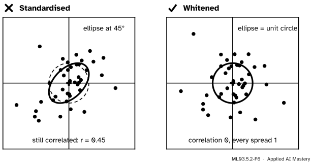
Wrong beside right. Standardising gives each feature spread 1 but leaves the correlation; only whitening makes the cloud round.
“Standardising the features whitens the data.”
Dividing each feature by its standard deviation (StandardScaler) sets the diagonal of the covariance to 1 and leaves the off-diagonal entries as the correlations. For the 40-point cloud the correlation stays at 0.45. In two dimensions the standardised covariance is
\[
\begin{bmatrix} 1 & r \\ r & 1 \end{bmatrix} ,
\]
whose eigenvectors lie along the diagonals, so the ellipse ends up at 45° when \(r > 0\) and at 135° when \(r < 0\), whatever the original tilt. Whitening also removes the correlation.
“Whitening is harmless: it only changes units.”
It divides each direction by \(\sqrt{\lambda_j}\), and the directions with tiny eigenvalues are often pure measurement noise. For the four points, a slip of 0.1 along \(\vect{q}_2\) becomes \({0.1/0.493 \approx 0.2}\) after whitening, while the same slip along \(\vect{q}_1\) shrinks to \({0.1/3.38 \approx 0.03}\). In high dimensions some \(\lambda_j\) are close to zero and the noise is blown up enormously. Whiten only the top \(q\) directions (PCA(n_components=q, whiten=True)) or add a small constant \(\varepsilon\) to each \(\lambda_j\) first.
“Classical MDS can draw any table of dissimilarities exactly.”
Only if the table holds Euclidean distances. Four towns on a ring road, 1 apart from each neighbour and 2 from the opposite town, cannot be placed in any space with those straight-line distances: the double-centred matrix has eigenvalue \(-1\), and a matrix \({\mat{X}_c\mat{X}_c\T}\) never has a negative eigenvalue. Classical MDS then keeps the positive part and the map is only an approximation. Check the sign of the eigenvalues you drop.
Check yourself
Recall
1. What two moves make up PCA whitening, and what is the whitened covariance?
Show answer
Rotate onto the principal axes with \(\mat{Q}\T\), then divide each coordinate by \(\sqrt{\lambda_j}\). The covariance becomes the identity.
2. How does ZCA whitening differ from PCA whitening?
Show answer
It rotates back with \(\mat{Q}\) after rescaling, so its matrix is \({\mat{C}^{-1/2}}\). The data stay in their original axes and move as little as possible.
3. When is the \({n \times n}\) matrix \({\mat{X}_c\mat{X}_c\T}\) the better route, and how do its eigenpairs give the scores?
Show answer
When \(d\) is much larger than \(n\). An eigenpair \({(\mu, \vect{u})}\) with unit \(\vect{u}\) gives the scores \({\sqrt{\mu}\,\vect{u}}\), and variance \({\mu/(n - 1)}\) along that direction.
4. What does double centring a matrix of squared Euclidean distances produce?
Show answer
\({-\tfrac12\mat{J}\mat{D}^{(2)}\mat{J} = \mat{X}_c\mat{X}_c\T}\), the dot products of the centred points.
5. What can classical MDS not recover from distances, and why?
Show answer
The orientation: a turn or a mirror image of the points leaves every distance unchanged, so the map is fixed only up to such a move (and a shift).
The point becomes \({(2/2,\; 3/3) = (1, 1)}\). With uncorrelated features, ZCA whitening is the same as standardising.
2.★★ Three towns have distances \({AB = 3}\), \({AC = 4}\) and \({BC = 5}\). Compute the entry \(b_{11}\) of the double-centred matrix and its trace, and check the trace against \({\sum_{i<j} D^{(2)}_{ij}/n}\).
Show solution
The squared distances are 9, 16 and 25. Row means of \({\mat{D}^{(2)}}\): \({(0 + 9 + 16)/3 = 25/3}\), \({(9 + 0 + 25)/3 = 34/3}\) and \({(16 + 25 + 0)/3 = 41/3}\); the overall mean is \({100/9}\). So
In the same way \({b_{22} = 52/9}\) and \({b_{33} = 73/9}\), so the trace is \({150/9 = 50/3}\). And \({(9 + 16 + 25)/3 = 50/3}\). (Placing A at the origin, B at \((3, 0)\) and C at \((0, 4)\), the centroid is \({(1, 4/3)}\) and \({b_{11} = 1 + 16/9 = 25/9}\), as it should be.)
3.★★★ Call \(\mat{W}\) a whitening matrix for \(\mat{C}\) if \({\mat{W}\mat{C}\mat{W}\T = \mat{I}}\). Show that every whitening matrix is \({\mat{R}\,\mat{C}^{-1/2}}\) for some orthogonal \(\mat{R}\).
Show solution
Let \({\mat{R} = \mat{W}\mat{C}^{1/2}}\). Then, using that \({\mat{C}^{1/2}}\) is symmetric,
so \(\mat{R}\) is orthogonal, and \({\mat{W} = \mat{R}\mat{C}^{-1/2}}\). Conversely any such product whitens, since \({\mat{R}\mat{C}^{-1/2}\mat{C}\mat{C}^{-1/2}\mat{R}\T = \mat{R}\mat{R}\T = \mat{I}}\). ZCA is \({\mat{R} = \mat{I}}\) and PCA whitening is \({\mat{R} = \mat{Q}\T}\).
Summary card
Whitening turns and stretches a cloud until it is round; double centring turns distances back into dot products.
Classical MDS.\({\mat{B} = -\tfrac12\mat{J}\mat{D}^{(2)}\mat{J}}\), then its top eigenpairs.
Sources and next steps
Sources. Each was opened and checked against this lesson on 15 November 2026.
Agnan Kessy, Alex Lewin and Korbinian Strimmer, Optimal whitening and decorrelation, The American Statistician 72 (2018), 309 to 314. Equations (1) to (3) define a whitening matrix by \({\mat{W}\T\mat{W} = \mat{\Sigma}^{-1}}\) and show it is not unique; equation (8) is ZCA whitening \({\mat{\Sigma}^{-1/2}}\) and (9) PCA whitening \({\mat{\Lambda}^{-1/2}\mat{U}\T}\), related by a rotation; Proposition 1 shows that ZCA minimises the expected squared distance between the whitened and the original vectors.
Christopher M. Bishop, Pattern Recognition and Machine Learning, Section 12.1.4, PCA for high-dimensional data: equations (12.26) to (12.30) derive the eigenvectors of the covariance from those of the \({N \times N}\) matrix and give their normalisation.
Trevor Hastie, Robert Tibshirani and Jerome Friedman, The Elements of Statistical Learning, corrected 12th printing, Section 14.8: classical scaling (14.100) works with centred inner products, is solved by eigenvectors (Exercise 14.11), and is exactly equivalent to principal components when the similarities are centred inner products.
scikit-learn 1.9, sklearn.decomposition.PCA (whiten=True gives uncorrelated outputs with unit variances) and sklearn.manifold.ClassicalMDS: for Euclidean distances, classical MDS is equivalent to PCA; metric="precomputed" takes a distance matrix.