A horizontal cut turns a dendrogram into clusters. Cut by height or by number of clusters, measure how faithfully the tree keeps the distances with the cophenetic correlation, and match SciPy’s fcluster and cophenet and scikit-learn’s AgglomerativeClustering.
ML03.2.3L2 Intermediate30 minIn review (what this means)
The maths and code on this page are checked by automated tests on every change, but an independent reader has not signed it off yet. Spot a mistake or a confusing step? Tell us.
Turn a dendrogram into a partition with a cut at height h, or with a cut that leaves K clusters.
Define the cophenetic distance, prove that it obeys the ultrametric inequality, and compute the cophenetic correlation from scratch.
Use scipy.cluster.hierarchy linkage, fcluster with the criteria ‘distance’ and ‘maxclust’, and cophenet, and match them with sklearn.cluster.AgglomerativeClustering.
Convert a Ward height in SciPy’s scale into the rise in the within-cluster sum of squares, and back.
The question
A tree is not yet an answer. A marketing team needs each customer in exactly one segment, and a lab needs each sample in one group. Where should the tree be cut, how do the libraries do it, and how can we tell whether the tree tells the truth about the distances it was built from?
From the last lesson
1. What does Ward’s linkage minimise at each merge, and in what scale does SciPy report it?
Show answer
The rise \(\Delta\) in the within-cluster sum of squares; SciPy reports the height \(\sqrt{2\Delta}\).
2. What are the complete-linkage merge heights of the values 1, 2, 4, 8, 11, 12?
Show answer
1, 1, 3, 4, 11.
Intuition
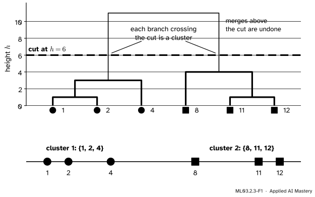
Draw a horizontal line across the dendrogram. Every merge below the line is kept and every merge above it is undone. The branches that the line crosses are the clusters, and the leaves hanging from each branch are its members.
ML03.2.3-F1
Cutting a dendrogram. The cut at \({h = 6}\) crosses two branches, so the tree becomes two clusters, \({\{1, 2, 4\}}\) and \({\{8, 11, 12\}}\). This tree is complete linkage, but every linkage of the last lesson gives the same two clusters here.
A low cut keeps few merges and gives many small clusters; a high cut gives a few large ones. Because the merge heights never decrease, sliding the line upwards only ever glues clusters together. That is the hierarchy at work: the clusters at one height are unions of the clusters at any lower height.
Build it up
Step 1. Cut at a height. Choose \(h\) and keep exactly the merges at height \(h\) or below. With \(n\) points and \(m\) merges kept, \({n - m}\) clusters remain.
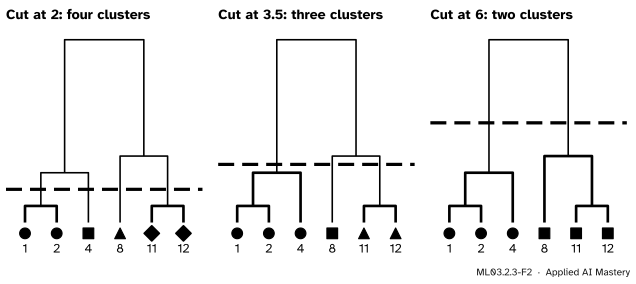
Step 2. Cut to a number of clusters. To get exactly \(K\) clusters, keep the first \({n - K}\) merges: put the line anywhere between the \({(n - K)}\)-th and the \({(n - K + 1)}\)-th merge heights.
ML03.2.3-F2
One tree, three cuts. Raising the line from 2 to 3.5 to 6 gives four, three and two clusters, and each clustering is made by gluing clusters of the one before.
Step 3. Choose where to cut. A tall stretch of the tree with no merges is a range of heights over which the clustering does not change; a cut in the middle of it is safe from small changes in the data. In the complete-linkage tree of the six values, the gap from 4 to 11 is by far the tallest, which points to two clusters. ESL puts it this way: groups that merge at high values, compared with the merges inside them, are candidates for natural clusters. It is a rule of thumb, and lesson ML03.10 gives sharper tools.
Step 4. Ask what the tree has kept. A dendrogram replaces the \({n(n - 1)/2}\) distances by \({n - 1}\) heights. For any two points, the tree’s own answer to “how far apart are they?” is the height at which they first share a cluster. Comparing those answers with the true distances tells us how faithful the tree is.
The formal statement
NoteDefinitions: cuts and cophenetic distances
Let the merges have heights \({h_1 \le h_2 \le \dots \le h_{n-1}}\).
The cut at height\(h\) is the partition into the clusters formed by the merges with \({h_t \le h}\). SciPy’s fcluster(Z, t, criterion="distance") gives it with \({t = h}\).
The cut into \(K\) clusters keeps the first \({n - K}\) merges. SciPy’s fcluster(Z, K, criterion="maxclust") finds the lowest cut with at most \(K\) clusters.
The cophenetic distance\(c_{ij}\) between points \(i\) and \(j\) is the height of the merge at which they first share a cluster.
The cophenetic correlation is the Pearson correlation between the \(d_{ij}\) and the \(c_{ij}\) over all \({n(n - 1)/2}\) pairs \({i < j}\).
So \({c_{ij} \le h}\) exactly when \(i\) and \(j\) are in the same cluster of the cut at \(h\): a cut at height \(h\) groups together the points whose cophenetic distance is at most \(h\). That is the wording of SciPy’s documentation for the "distance" criterion.
Written out, with \(\bar d\) and \(\bar c\) the means over the pairs,
\[
r = \frac{S_{dc}}{\sqrt{S_{dd}\, S_{cc}}}, \quad \text{where}
\]
A value near 1 means the tree keeps the pattern of the distances well. It cannot reach 1 on most data, for a reason that the next result makes precise: cophenetic distances are a very special kind of distance.
Cophenetic distances are ultrametric. For any three points \(i\), \(j\) and \(k\),
\[
c_{ij} \le \max(c_{ik},\, c_{jk}).
\]
Proof. Let \({m = \max(c_{ik}, c_{jk})}\) and look at the clustering after all merges of height at most \(m\). Since \({c_{ik} \le m}\), points \(i\) and \(k\) are in the same cluster. Since \({c_{jk} \le m}\), points \(j\) and \(k\) are in the same cluster. A point belongs to only one cluster at a time, so both clusters are the one holding \(k\), and \(i\) and \(j\) are together. So they first shared a cluster at a height of at most \(m\): \({c_{ij} \le m}\). \(\square\)
In words, of the three cophenetic distances among any three points, the two largest are equal. Real distances rarely behave like that, which is why ESL calls the cophenetic distance a very restrictive dissimilarity, with at most \({n - 1}\) distinct values among \({n(n - 1)/2}\) pairs.
Worked example
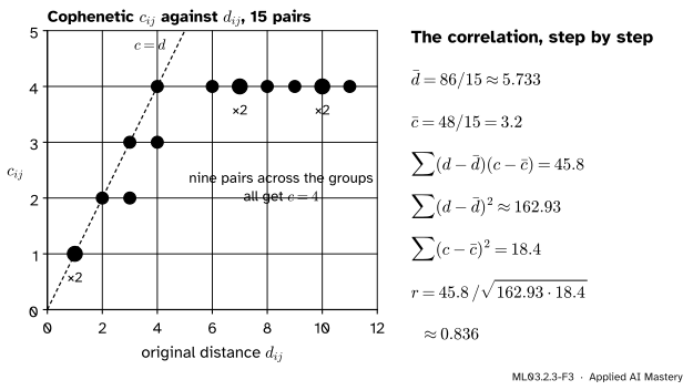
The cophenetic correlation of the six values under single linkage. The heights are 1, 1, 2, 3, 4 (lesson ML03.2.1). Read each pair’s cophenetic distance off the tree:
\({c = 1}\) for the pairs \({(1, 2)}\) and \({(11, 12)}\), whose distances are 1 and 1;
\({c = 2}\) for \({(1, 4)}\) and \({(2, 4)}\), distances 3 and 2;
\({c = 3}\) for \({(8, 11)}\) and \({(8, 12)}\), distances 3 and 4;
\({c = 4}\) for the nine pairs across the two groups, distances 7, 10, 11, 6, 9, 10, 4, 7, 8.
The means are \({\bar d = 86/15 \approx 5.733}\) and \({\bar c = 48/15 = 3.2}\). The three sums come to \({S_{dc} = 45.8}\), \({S_{dd} \approx 162.93}\) and \({S_{cc} = 18.4}\), so
\[
r = \frac{45.8}{\sqrt{162.93 \times 18.4}} \approx 0.836 .
\]
ML03.2.3-F3
The tree’s distances against the true ones. Single linkage flattens every distance across the two groups, from 4 to 11, to the one height 4, and that costs it correlation.
The other linkages keep more: complete 0.864, Ward 0.862 and average 0.865, the highest here, though on these six values the four are close.
Code
A cut from scratch is a union of the merges kept, and the cophenetic distances are filled in merge by merge: every pair split across the two parts of a merge gets that merge’s height.
import numpy as npfrom scipy.cluster.hierarchy import cophenet, fcluster, linkagefrom scipy.spatial.distance import pdistdef cut(Z, keep):"""Cluster labels after keeping the first `keep` merges of a SciPy linkage matrix.""" n =len(Z) +1 members = {i: [i] for i inrange(n)}for t inrange(keep): a, b =int(Z[t, 0]), int(Z[t, 1]) members[n + t] = members.pop(a) + members.pop(b) labels = np.empty(n, dtype=int)for k, group inenumerate(members.values()): labels[group] = kreturn labelsdef cut_at_height(Z, h):return cut(Z, int(np.sum(Z[:, 2] <= h)))def cut_into(Z, K):return cut(Z, len(Z) +1- K)def cophenetic(Z): n =len(Z) +1 members = {i: [i] for i inrange(n)} C = np.zeros((n, n))for t inrange(len(Z)): A, B = members.pop(int(Z[t, 0])), members.pop(int(Z[t, 1])) C[np.ix_(A, B)] = Z[t, 2] C[np.ix_(B, A)] = Z[t, 2] members[n + t] = A + Breturn C[np.triu_indices(n, 1)] # the same pair order as pdistvalues = np.array([1, 2, 4, 8, 11, 12]).reshape(-1, 1)d = pdist(values)for method in ["single", "complete", "average", "ward"]: Z = linkage(values, method) r = np.corrcoef(d, cophenetic(Z))[0, 1]print(f"{method:9s} two clusters: {cut_into(Z, 2)} cophenetic correlation {r:.3f}")
single    two clusters: [0 0 0 1 1 1]  cophenetic correlation 0.836
complete  two clusters: [0 0 0 1 1 1]  cophenetic correlation 0.864
average   two clusters: [0 0 0 1 1 1]  cophenetic correlation 0.865
ward      two clusters: [0 0 0 1 1 1]  cophenetic correlation 0.862
SciPy’s cophenet returns the same correlation and distances, and fcluster makes both kinds of cut. Note that t means a height under "distance" and a number of clusters under "maxclust".
Z = linkage(values, "single")print("cophenet: ", round(cophenet(Z, d)[0], 3))print("distance, t = 2: ", fcluster(Z, 2, criterion="distance"))print("maxclust, t = 2: ", fcluster(Z, 2, criterion="maxclust"))print("ours, height 2: ", cut_at_height(Z, 2))
scikit-learn’s AgglomerativeClustering cuts to a number of clusters, or at a height with distance_threshold. With compute_distances=True it also returns the merge heights, and for Ward they are in SciPy’s scale, so \({\Delta = h^2/2}\).
from sklearn.cluster import AgglomerativeClusteringfor method in ["single", "complete", "average", "ward"]: model = AgglomerativeClustering(n_clusters=2, linkage=method, compute_distances=True).fit(values)print(f"{method:9s} labels {model.labels_} heights {np.round(model.distances_, 3)}")ward = AgglomerativeClustering(n_clusters=2, linkage="ward", compute_distances=True).fit(values)print("Ward rises in the sum of squares:", np.round(ward.distances_ **2/2, 4))
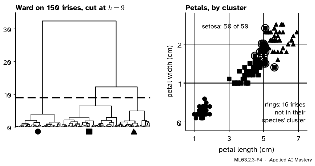
Finally the 150 irises of load_iris, four measurements in centimetres. Ward linkage cut into three clusters, compared with the species, which the clustering never saw:
from sklearn.datasets import load_irisX, species = load_iris(return_X_y=True)Zi = linkage(X, "ward")clusters = fcluster(Zi, 3, criterion="maxclust")table = np.zeros((3, 3), dtype=int)for k, s inzip(clusters, species): table[k -1, s] +=1print("rows: clusters; columns: setosa, versicolor, virginica")print(table)print("cophenetic correlations:", {m: round(float(cophenet(linkage(X, m), pdist(X))[0]), 3) for m in ["single", "complete", "average", "ward"]})
Ward linkage on load_iris, cut into three clusters. Setosa is found exactly; versicolor and virginica overlap, and 16 of the 150 irises land in the cluster where the other species is the majority.
Setosa comes out exactly. One cluster holds 49 versicolor and 15 virginica, the other 35 virginica and 1 versicolor, so 134 of the 150 irises share a cluster with most of their species. Average linkage has the highest cophenetic correlation here, 0.877, and complete the lowest, 0.727. (load_iris has a repeated row and many tied distances, and the order in which tied merges are taken matters: shuffling the rows moves the complete-linkage value between about 0.727 and 0.728.)
Explore
ML03.2-X1
Dendrogram cutter
Load the six values, the nine points or the twelve points, or drag up to twelve points of your own. Choose a linkage, press Step to merge one pair at a time, and drag the orange cut line (or use its slider) to colour the clusters it makes. Watch the cophenetic correlation as you switch linkage.
Pitfalls
ML03.2.3-F5
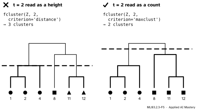
Wrong beside right, if two clusters were wanted. Under "distance", t = 2 is a height, and a cut at height 2 leaves three clusters. Under "maxclust", t = 2 is a number of clusters.
“fcluster(Z, 2) gives me two clusters.”
Its default criterion is neither of the two above but "inconsistent", a third rule, and under "distance" the 2 is a height. Always name the criterion. The cut at height 2 also shows a second trap: it sits exactly on a merge, and "distance" keeps merges at height at most\(t\), so the answer depends on that “at most”. Cut in the middle of a gap between heights, never on one.
“A high cophenetic correlation means good clusters.”
It measures how well the tree keeps the pattern of all the distances, small and large. A tree can keep them well and still be cut into clusters that mean nothing, and uniform noise with no clusters at all still gets a tree and a correlation. Use it to compare linkages on the same data, and judge the clusters with the tools of ML03.10.
“A Ward distance_threshold is a distance between points.”
For Ward linkage both SciPy and scikit-learn measure heights as \(\sqrt{2\Delta}\), which grows with the sizes of the clusters, so a threshold of 5 does not mean “points within 5 of each other”. To stop merging when a merge would raise the sum of squares by more than \(\Delta^\star\), cut at \(\sqrt{2\Delta^\star}\).
Check yourself
Recall
1. How many clusters does a cut at height \(h\) leave, in terms of the merges?
Show answer
\({n - m}\), where \(m\) is the number of merges with height at most \(h\).
2. Define the cophenetic distance \(c_{ij}\).
Show answer
The height of the merge at which points \(i\) and \(j\) first share a cluster.
3. State the ultrametric inequality that cophenetic distances obey.
Show answer
\({c_{ij} \le \max(c_{ik}, c_{jk})}\) for any three points \(i\), \(j\), \(k\).
4. What does t mean in fcluster(Z, t, criterion="distance"), and in criterion="maxclust"?
Show answer
Under "distance" it is a height: merges at height at most \(t\) are kept. Under "maxclust" it is the largest number of clusters wanted.
5. Under single linkage, what is the cophenetic correlation of the six values?
Show answer
About 0.836.
Exercises
1.★ Using the average-linkage heights of the six values (1, 1, 2.5, 3.5, 8), give the clusters for cuts at \({h = 3}\) and \({h = 5}\), and a range of heights that gives four clusters.
Show solution
At \({h = 3}\) three merges are kept (1, 1, 2.5): \({\{1, 2, 4\}}\), \(\{8\}\), \({\{11, 12\}}\). At \({h = 5}\) four are kept: \({\{1, 2, 4\}}\) and \({\{8, 11, 12\}}\). Four clusters need exactly \({6 - 4 = 2}\) merges, so any \(h\) with \({1 \le h < 2.5}\), giving \({\{1, 2\}}\), \(\{4\}\), \(\{8\}\), \({\{11, 12\}}\).
2.★★ Write down the cophenetic distances of the six values under complete linkage and compute \(\bar c\). Which pairs have \({c_{ij} = 11}\)?
Show solution
With heights 1, 1, 3, 4, 11: \({c = 1}\) for \({(1, 2)}\) and \({(11, 12)}\); \({c = 3}\) for \({(1, 4)}\) and \({(2, 4)}\); \({c = 4}\) for \({(8, 11)}\) and \({(8, 12)}\); and \({c = 11}\) for the nine pairs with one value in \({\{1, 2, 4\}}\) and the other in \({\{8, 11, 12\}}\). Then
3.★★★ The single-linkage and average-linkage trees of the six values merge the same clusters in the same order. Show that they give the same clusters for every \(K\), yet different cophenetic correlations, and explain which tree keeps the distances better.
Show solution
A cut into \(K\) clusters keeps the first \({6 - K}\) merges, and which merges those are does not depend on their heights, only on their order. Both trees make the same merges in the same order, so they give the same partition for every \(K\). A pair’s cophenetic distance is the height of the merge that first joins it, so the cophenetic distances do depend on the heights. Their heights differ, 1, 1, 2, 3, 4 against 1, 1, 2.5, 3.5, 8, so the cophenetic distances differ, and the correlations are 0.836 and 0.865. The average tree stretches the cross-group pairs to 8, closer to their true distances of 4 to 11, and so keeps the distances better.
Summary card
A horizontal cut turns the tree into clusters; the cophenetic correlation says how faithful the tree is.
ML03.2.3-F1
Cut in a tall gap.
Cut at \(h\): keep merges with height at most \(h\) (fcluster(..., criterion="distance")).
Cut into \(K\): keep the first \({n - K}\) merges (criterion="maxclust").
Cophenetic distance\(c_{ij}\): height of the first common merge; \({c_{ij} \le \max(c_{ik}, c_{jk})}\).
Cophenetic correlation: Pearson \(r\) of \(d_{ij}\) and \(c_{ij}\); single linkage on the six values: 0.836.
Ward heights:\({h = \sqrt{2\Delta}}\), so \({\Delta = h^2/2}\).
Sources and next steps
Sources. Each was opened and checked against this lesson on 15 November 2026.
G. James, D. Witten, T. Hastie and R. Tibshirani, An Introduction to Statistical Learning, 2nd edition. Section 12.4.2: a horizontal cut gives the clusters below it; cuts at heights nine and five give two and three clusters in Figure 12.11; the height of the cut plays the role of \(K\); the clusters at one height are nested in those at any greater height.
T. Hastie, R. Tibshirani and J. Friedman, The Elements of Statistical Learning, 2nd edition, 12th printing. Section 14.3.12: cutting at a threshold, groups that merge at high values as candidates for natural clusters, the cophenetic correlation coefficient, and the ultrametric inequality (14.40) with at most \({N - 1}\) distinct cophenetic values.
SciPy developers, scipy.cluster.hierarchy.fcluster and cophenet: the default criterion "inconsistent"; "distance" keeps cophenetic distances no greater than t; "maxclust" finds the lowest threshold with at most t clusters; cophenet returns the correlation and the condensed cophenetic distances.
scikit-learn developers, sklearn.cluster.AgglomerativeClustering (version 1.9): Ward as the default linkage, distance_threshold, compute_distances and distances_, and children_ in the order of the merges.