A cluster is a crowd of points separated from other crowds by sparse ground, whatever its shape. Learn the definitions of DBSCAN (core, border and noise points, and reachability), run it by hand on the twelve points, and build it as a breadth-first search.
ML03.3.1L2 Intermediate30 minIn review (what this means)
The maths and code on this page are checked by automated tests on every change, but an independent reader has not signed it off yet. Spot a mistake or a confusing step? Tell us.
Define the eps-neighbourhood, core, border and noise points, and decide which each point of a small data set is.
Explain direct density-reachability, density-reachability and density-connectedness, and why only the last is symmetric.
Run DBSCAN by hand on the twelve points with eps = 1.5 and min_samples = 4, and get two clusters of five and two noise points.
Build DBSCAN from scratch as a breadth-first search over core points and match sklearn.cluster.DBSCAN.
The question
k-means asks for the number of clusters, cuts every cluster into a round cell around a centre, and puts every single point somewhere, strays included. Look at a map of where taxis pick people up, or at two interleaved half-moons, and none of that fits: the groups have odd shapes, nobody told you how many there are, and some points belong to no group at all. Can an algorithm find crowds of any shape and leave the strays out?
Intuition
Think of the points as people in a field. A cluster is a crowd, separated from other crowds by open ground where people stand thinly. To find the crowds you need no centres, only one question for each person: how many people stand within arm’s reach of you?
ML03.3.1-F1
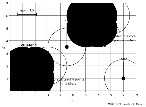
DBSCAN on the twelve points with \(\varepsilon = 1.5\) and four points per circle. Core points (large) have at least four points within \(\varepsilon\), themselves included. Border points (small) have fewer, but sit in a core point’s circle. Noise points (rings) have neither.
Fix a radius \(\varepsilon\) (“eps” in code) and a count \(m\) (“min_samples”). A point with at least \(m\) points inside its circle of radius \(\varepsilon\) is in the middle of a crowd: a core point. A point with fewer, but which sits inside the circle of some core point, is on the edge of a crowd: a border point. Everything else is noise. Then let each crowd spread: a core point passes its cluster on to every point in its circle, and any core point reached that way passes it on again.
This is DBSCAN (density-based spatial clustering of applications with noise), from Ester, Kriegel, Sander and Xu (1996). The number of clusters comes out of the data.
Build it up
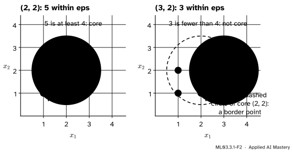
Step 1. Count the neighbours. Around each point, draw the circle of radius \(\varepsilon = 1.5\) and count the points inside it, the point itself included. For the corner \((2, 2)\) of the lower square, the other three corners are at distances \(1\), \(1\) and \(\sqrt{2} \approx 1.414\), and \((3, 2)\) is at distance \(1\). With itself, that makes 5.
ML03.3.1-F2
Counting within \(\varepsilon\). The corner \((2, 2)\) has 5 points in its circle, so it is core. The point \((3, 2)\) has only 3, so it is not core; but it lies in the circle of the core point \((2, 2)\), which makes it a border point.
Step 2. Mark the core points. With \(m = 4\), the point \((2, 2)\) is core. The point \((3, 2)\) counts only itself, \((2, 1)\) and \((2, 2)\): three, which is too few.
Step 3. Let the core points reach out. A core point reaches every point in its circle. The corner \((2, 2)\) reaches \((3, 2)\). The reverse fails: \((3, 2)\) is not core, so it reaches nothing, even though \((2, 2)\) lies in its circle.
Step 4. Follow chains. Clusters spread through chains of core points. Starting from \((1, 1)\), the cluster passes to \((2, 1)\), which is core, so it passes on to \((3, 2)\). The point \((3, 2)\) joins as a border point, and the chain stops there.
Step 5. Whatever no chain reaches is noise. The bridge point \((4.5, 3.5)\) has no other point within \(1.5\): its nearest neighbours are \(\sqrt{4.5} \approx 2.121\) away.
The formal statement
Let \(D\) be a set of \(n\) points with a distance \(d\), and fix \(\varepsilon > 0\) and a whole number \(m \ge 1\). The definitions follow Ester et al. (1996, section 3).
NoteDefinitions: the language of DBSCAN
The \(\varepsilon\)-neighbourhood\(N_\varepsilon(\vect{p})\) of a point \(\vect{p}\) is the set of points of \(D\) within distance \(\varepsilon\) of it. It contains \(\vect{p}\) itself.
\(\vect{p}\) is a core point if \(\abs{N_\varepsilon(\vect{p})} \ge m\).
\(\vect{q}\) is directly density-reachable from \(\vect{p}\) if \(\vect{p}\) is a core point and \(\vect{q} \in N_\varepsilon(\vect{p})\).
\(\vect{q}\) is density-reachable from \(\vect{p}\) if there is a chain of points from \(\vect{p}_1 = \vect{p}\) to \(\vect{p}_k = \vect{q}\) in which each point is directly density-reachable from the one before.
\(\vect{p}\) and \(\vect{q}\) are density-connected if both are density-reachable from some third point \(\vect{o}\).
A cluster is a non-empty set \(C\) that is maximal (if \(\vect{p} \in C\) and \(\vect{q}\) is density-reachable from \(\vect{p}\), then \(\vect{q} \in C\)) and connected (any two of its points are density-connected). Noise is every point that belongs to no cluster.
In symbols, the neighbourhood and the core condition are
\[
\begin{aligned}
N_\varepsilon(\vect{p}) &= \{\vect{q} \in D : d(\vect{p}, \vect{q}) \le \varepsilon\}, \\
\vect{p} \text{ is core} &\iff \abs{N_\varepsilon(\vect{p})} \ge m .
\end{aligned}
\]
A border point is a point of a cluster that is not core. scikit-learn’s min_samples is \(m\), and it counts the point itself, as the definition of \(N_\varepsilon\) does.
Why reachability is not symmetric. In a chain, every point except possibly the last must be core, since each link starts at a core point. So a border point can be reached, but nothing can be reached from it. That is why the definition of a cluster needs density-connectedness: two border points of the same crowd cannot reach each other, but both are reached from a core point between them.
Between core points, reachability is symmetric. Suppose \(\vect{p}\) and \(\vect{q}\) are both core and \(d(\vect{p}, \vect{q}) \le \varepsilon\). Then \(\vect{q} \in N_\varepsilon(\vect{p})\) and \(\vect{p}\) is core, so \(\vect{q}\) is directly reachable from \(\vect{p}\); and since distance is symmetric, the same argument run the other way gives \(\vect{p}\) from \(\vect{q}\). Reverse a chain of core points link by link and you get a chain back.
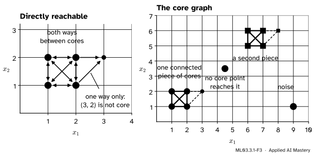
This gives a clean picture of the result. Join two core points by an edge when they are within \(\varepsilon\) of each other: call it the core graph.
ML03.3.1-F3
Left: direct reachability runs both ways between core points, and only outwards to a border point. Right: a cluster is one connected piece of the core graph, together with the border points within \(\varepsilon\) of it.
NoteResult: what DBSCAN returns
The clusters are exactly the connected pieces of the core graph, each together with the non-core points that lie within \(\varepsilon\) of one of its core points. The rest is noise.
The algorithm that finds them is a breadth-first search. Visit the points in turn. When you meet a core point that has no label yet, start a new cluster, give it the label and put it in a queue. Then repeat: take a point from the queue; if it is core, give the label to every unlabelled point in its neighbourhood and add them to the queue. When the queue is empty, the cluster is complete. This is Lemma 2 of Ester et al.: a cluster is the set of points density-reachable from any one of its core points, so it does not matter which core point you start from.
Go deeper: why the breadth-first search returns exactly the clusters
Start the search at a core point \(\vect{p}\). Every point it labels is reached through a chain of core points that begins at \(\vect{p}\), so it is density-reachable from \(\vect{p}\). Conversely, a point \(\vect{q}\) that is density-reachable from \(\vect{p}\) has a chain from \(\vect{p}_1 = \vect{p}\) to \(\vect{p}_k = \vect{q}\) whose links all start at core points. By induction along the chain, the search puts each \(\vect{p}_i\) in the queue, and since \(\vect{p}_i\) is core for \(i < k\), it labels \(\vect{p}_{i+1}\) when it takes \(\vect{p}_i\) out. So the search labels exactly the set of points density-reachable from \(\vect{p}\), which is a cluster by Lemma 1 of the paper.
One subtlety remains: a border point can lie within \(\varepsilon\) of core points of two different clusters. It then belongs to both by the definition, and the search gives it to whichever cluster reaches it first. The next lesson shows that case on the twelve points.
Worked example
The twelve points with \(\varepsilon = 1.5\) and \(m = 4\). The points are \((1, 1)\), \((2, 1)\), \((1, 2)\), \((2, 2)\), \((3, 2)\), \((6, 5)\), \((7, 5)\), \((6, 6)\), \((7, 6)\), \((8, 6)\), \((4.5, 3.5)\) and \((9, 1)\).
Neighbour counts. Within a square of side 1 every corner sees the other three: two at distance 1 and one at \(\sqrt{2} \approx 1.414\), all within 1.5. The extra point \((3, 2)\) is within 1.5 of \((2, 1)\) (distance \(\sqrt{2}\)) and \((2, 2)\) (distance 1), but not of \((1, 2)\) (distance 2). So the counts, the point itself included, are 4, 5, 4 and 5 for \((1, 1)\), \((2, 1)\), \((1, 2)\), \((2, 2)\), and 3 for \((3, 2)\). The upper group has the same shape, shifted by \((5, 4)\), so its counts are the same: 4, 5, 4, 5 and 3 for \((8, 6)\). The bridge point and \((9, 1)\) count 1 each.
Core points. Count at least 4: the eight corners of the two squares.
ML03.3.1-F4
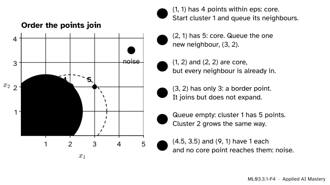
The breadth-first search, step by step. The numbers on the left show the order in which points join cluster 1.
The search. The first point, \((1, 1)\), is core: it starts cluster 1, and its three neighbours join the queue. Taking out \((2, 1)\), which is core, adds its one new neighbour \((3, 2)\). Nothing else is new, and \((3, 2)\), not being core, does not spread the label. The next unlabelled core point, \((6, 5)\), grows cluster 2 in the same way, ending with the border point \((8, 6)\).
Result: two clusters of five, core points the two squares, border points \((3, 2)\) and \((8, 6)\), noise \((4.5, 3.5)\) and \((9, 1)\).
Code
First from scratch. The neighbour lists come from the matrix of all pairwise distances, and the search is the queue of the formal statement.
from collections import dequeimport numpy as npX = np.array([(1, 1), (2, 1), (1, 2), (2, 2), (3, 2), (6, 5), (7, 5), (6, 6), (7, 6), (8, 6), (4.5, 3.5), (9, 1)], dtype=float)def dbscan(X, eps, min_samples):"""Labels 0, 1, ... for clusters and -1 for noise, and a mask of the core points.""" D = np.sqrt(((X[:, None, :] - X[None, :, :]) **2).sum(axis=-1)) neighbours = [np.flatnonzero(row <= eps) for row in D] # each includes the point itself core = np.array([len(nb) >= min_samples for nb in neighbours]) labels = np.full(len(X), -1) cluster =-1for i inrange(len(X)):if labels[i] !=-1ornot core[i]:continue cluster +=1# a new cluster starts here labels[i] = cluster queue = deque([i])while queue: p = queue.popleft()ifnot core[p]:continue# border points do not spreadfor q in neighbours[p]:if labels[q] ==-1: labels[q] = cluster queue.append(q)return labels, corecounts = [int((np.sqrt(((X - x) **2).sum(axis=1)) <=1.5).sum()) for x in X]labels, core = dbscan(X, eps=1.5, min_samples=4)print("neighbour counts:", counts)print("labels:", labels)print("core points:", np.flatnonzero(core))
Now scikit-learn, whose min_samples also counts the point itself. labels_ uses \(-1\) for noise, and core_sample_indices_ lists the core points.
from sklearn.cluster import DBSCANdb = DBSCAN(eps=1.5, min_samples=4).fit(X)print("labels_:", db.labels_)print("core_sample_indices_:", db.core_sample_indices_)border = [i for i inrange(len(X)) if db.labels_[i] >=0and i notin db.core_sample_indices_]print("border points:", X[border].tolist())
The distance matrix holds \(n^2\) numbers; for large data scikit-learn finds neighbourhoods with a tree instead.
Explore
This module’s interactive, the DBSCAN explorer, lives in the next lesson: slide \(\varepsilon\) and min_samples on these twelve points and watch each point relabel itself.
Pitfalls
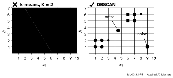
ML03.3.1-F5
Wrong beside right. k-means must give every point a cluster, so the two strays are pulled into the upper group and drag its centre towards them. DBSCAN leaves them out as noise.
“Every point must end up in some cluster.”
That is a habit from k-means, not a law. Forcing measurement errors and one-off visitors into a cluster mislabels them and moves the cluster. DBSCAN’s \(-1\) label is information: its noise points are the first candidates to inspect, a link that anomaly detection (ML03.9) develops.
“Treat label \(-1\) as one more cluster.”
Noise points share nothing but being alone. Averaging them, or scoring them as a cluster (ML03.10.1), describes a group that does not exist. Drop them, and report their number separately.
“min_samples = 4 means four neighbours.”
In the paper and in scikit-learn the count includes the point itself, so min_samples = 4 means three other points within \(\varepsilon\). The separate hdbscan library counts only the others, so check before you move a setting between libraries.
Check yourself
Recall
1. What makes a point a core point?
Show answer
At least \(m\) (min_samples) points within distance \(\varepsilon\) of it, the point itself included.
2. What is the difference between a border point and a noise point?
Show answer
Neither is core. A border point lies within \(\varepsilon\) of some core point, so it belongs to that point’s cluster. A noise point lies within \(\varepsilon\) of no core point and belongs to no cluster.
3. Why is density-reachability not symmetric?
Show answer
Every link of a chain must start at a core point. A border point can be reached from a core point, but it reaches nothing itself, so the chain cannot be walked back from it.
4. In the twelve points with \(\varepsilon = 1.5\) and \(m = 4\), which points are border points and which are noise?
Show answer
Border: \((3, 2)\) and \((8, 6)\). Noise: \((4.5, 3.5)\) and \((9, 1)\).
5. What label does sklearn.cluster.DBSCAN give noise, and which attribute lists the core points?
Show answer
Noise gets the label \(-1\) in labels_. The core points are listed in core_sample_indices_.
Exercises
1.★ Rerun the twelve points with \(\varepsilon = 1.5\) but min_samples = 3, then with min_samples = 6. Which points are core each time, and what are the clusters?
Show solution
The neighbour counts are 4, 5, 4, 5, 3 in each group, and 1 for the bridge and \((9, 1)\).
With \(m = 3\), every point with a count of at least 3 is core: all ten points of the two groups. The clusters are the same two groups of five, and the bridge and \((9, 1)\) are still noise, since their count is 1.
With \(m = 6\), no count reaches 6, so there are no core points at all. No cluster can start, and all twelve points are noise.
2.★★ Add the point \((4, 3)\) to the twelve points, keeping \(\varepsilon = 1.5\) and \(m = 4\). Work out its neighbour count and the new count of the bridge point, and say what DBSCAN returns now.
Show solution
Distances from \((4, 3)\): to \((3, 2)\) it is \(\sqrt{2} \approx 1.414\); to the bridge \((4.5, 3.5)\) it is \(\sqrt{0.5} \approx 0.707\); to \((2, 2)\) it is \(\sqrt{5} \approx 2.236\); to \((6, 5)\) it is \(\sqrt{8} \approx 2.828\). So its neighbourhood is itself, \((3, 2)\) and the bridge: a count of 3, not core.
The bridge now has itself and \((4, 3)\) within 1.5: a count of 2, still not core.
The point \((3, 2)\) gains \((4, 3)\) and now counts 4: it becomes core. As a core point it reaches \((4, 3)\), which joins cluster 1 as a border point. The bridge is \(\sqrt{4.5} \approx 2.121\) from \((3, 2)\), too far to be reached, and \((4, 3)\) is not core, so the chain stops. Result: cluster 1 has six points, cluster 2 has five, and the bridge and \((9, 1)\) are noise.
3.★★★ Let \(\vect{p}\) and \(\vect{q}\) be two core points that are density-connected. Show that \(\vect{q}\) is density-reachable from \(\vect{p}\), so that among core points the three notions of reachability coincide.
Show solution
Density-connected means there is a point \(\vect{o}\) with two chains, each link directly density-reachable:
Every link starts at a core point, so \(\vect{a}_1, \dots, \vect{a}_{k-1}\) are core; and \(\vect{a}_k = \vect{p}\) is core by assumption. So the whole first chain consists of core points, each within \(\varepsilon\) of the next.
Between two core points within \(\varepsilon\) of each other, direct reachability holds both ways (shown in the formal statement). Reverse the first chain link by link, from \(\vect{a}_k = \vect{p}\) back to \(\vect{a}_1 = \vect{o}\): it is a valid chain, so \(\vect{o}\) is density-reachable from \(\vect{p}\). Append the second chain, which starts at \(\vect{o}\): the result runs from \(\vect{p}\) to \(\vect{q}\), with every link starting at a core point. So \(\vect{q}\) is density-reachable from \(\vect{p}\).
This is why the core points of a cluster form one connected piece of the core graph.
Summary card
A cluster is a crowd: core points within reach of each other, plus their border points.
ML03.3.1-F1
Core, border and noise.
Neighbourhood.\(N_\varepsilon(\vect{p})\): the points within \(\varepsilon\) of \(\vect{p}\), itself included.
Core.\(\abs{N_\varepsilon(\vect{p})} \ge m\). Border: not core, but within \(\varepsilon\) of a core point. Noise: neither.
Clusters. Connected pieces of the core graph, plus their border points; found by breadth-first search.
In code.DBSCAN(eps, min_samples).fit(X): labels_ with \(-1\) for noise, core_sample_indices_.
Sources and next steps
Sources. Each was opened and checked against this lesson on 15 November 2026.
Martin Ester, Hans-Peter Kriegel, Jörg Sander and Xiaowei Xu, A density-based algorithm for discovering clusters in large spatial databases with noise, KDD-96, pages 226 to 231. Section 3 gives Definitions 1 to 6 (Eps-neighbourhood, directly density-reachable with the core point condition, density-reachable, density-connected, cluster, noise) and Lemmas 1 and 2 (a cluster is what is density-reachable from any of its core points); section 4.1 gives the algorithm with its seed list.
scikit-learn developers, User Guide, section 2.3.7 DBSCAN, version 1.9: core samples, border (non-core) samples and outliers, and memory use without a tree.
scikit-learn developers, sklearn.cluster.DBSCAN: min_samples includes the point itself; labels_ gives \(-1\) for noise; core_sample_indices_.
scikit-learn developers, sklearn.cluster.HDBSCAN, Notes: the hdbscan library’s min_samples does not count the point.