Give every document’s topic shares a Dirichlet prior and the topic model can generate, and score, any document. Meet the Dirichlet on a triangle, derive the collapsed Gibbs update as a product of two counts, and fit topics from scratch and with scikit-learn.
ML03.7.4L2 Intermediate25 minIn review (what this means)
The maths and code on this page are checked by automated tests on every change, but an independent reader has not signed it off yet. Spot a mistake or a confusing step? Tell us.
Tell the generative story of latent Dirichlet allocation and say what the priors on the topic shares and on the topics add to pLSA.
Describe how the Dirichlet concentration shapes proportions on the triangle of three topics.
State the collapsed Gibbs update for one word’s topic, compute it from counts by hand, and derive it from the Dirichlet integrals.
Fit the topic model from scratch and with LatentDirichletAllocation, read topics by their top words, and choose K by held-out perplexity.
The question
A new document arrives: “goal oven”. pLSA has no topic shares for it, because its shares were parameters fitted to the training documents, one set each. How can a topic model give any document, seen or unseen, a probability, and stop growing a new set of parameters for every page of text it reads?
From the last lesson
1. What does the pLSA E-step compute for a word \(w\) in document \(d\)?
Show answer
The responsibility of each topic, \({r_{dwk} \propto P(k \mid d)\,P(w \mid k)}\), by Bayes’ rule.
2. Why can pLSA not score a new document?
Show answer
Its topic shares \({P(k \mid d)}\) exist only for training documents; \(d\) is an index into the training set, so the model does not generate new documents.
Intuition
Keep pLSA’s story of topics choosing words, and add one step at the top: every document draws its topic shares at random from a common distribution. Now the shares are not parameters to fit, one set per document, but random quantities the model can average over.
ML03.7.4-F1
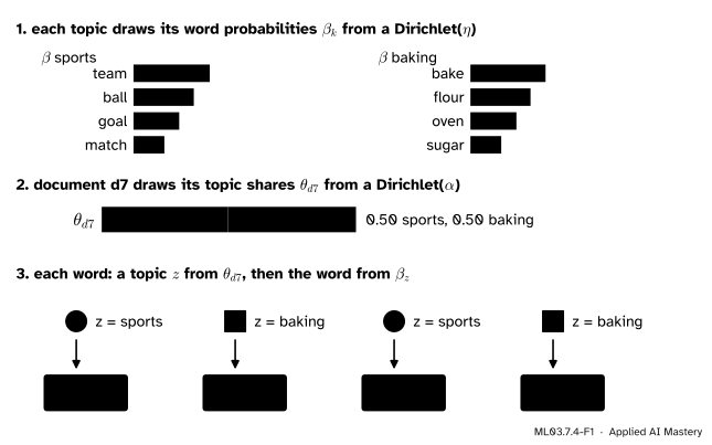
The generative story of the topic model, told for d7. Topics are drawn once for the corpus, topic shares once per document, and a topic and a word for every word.
This is latent Dirichlet allocation (Blei, Ng and Jordan, 2003). We call it the topic model here, because in this course the letters LDA belong to linear discriminant analysis. The letters follow theirs: \(K\) topics, topic shares \(\vect{\theta}_d\) for document \(d\), and word probabilities \(\vect{\beta}_k\) for topic \(k\).
Build it up
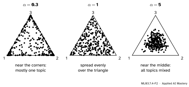
Step 1. A distribution over proportions. The topic shares of a document are \(K\) numbers that are at least 0 and add to 1: a point on the simplex. With three topics the simplex is a triangle, each corner a document of one pure topic. The Dirichlet distribution with concentration \({\alpha > 0}\) (the same for every topic) has density
on the simplex, where \(\Gamma\) is the gamma function (\({\Gamma(n) = (n - 1)!}\) for whole \(n\)). Its mean is \({1/K}\) for every topic. The concentration sets how spread out the shares are.
ML03.7.4-F2
Three hundred draws from a Dirichlet for three concentrations. Below 1 a document leans to one topic; at 1 every mix is equally likely; above 1 documents mix all topics.
Read the exponent \({\alpha - 1}\): below 1 the density blows up near the edges, where some \({\theta_{dk}}\) is near 0, and above 1 it vanishes there. Real documents are about a few things, so topic models usually use \({\alpha < 1}\).
Step 2. The whole story. For a corpus with \(K\) topics and \(V\) words:
For each topic \(k\), draw word probabilities \({\vect{\beta}_k \sim \text{Dirichlet}(\eta)}\).
For each document \(d\), draw topic shares \({\vect{\theta}_d \sim \text{Dirichlet}(\alpha)}\).
For each word of \(d\), draw a topic \({z \sim \vect{\theta}_d}\), then the word from \({\vect{\beta}_z}\).
The prior \(\eta\) on the topics smooths them, so a word never seen in a topic still has a small probability (Blei, Ng and Jordan’s section 5.4). The prior \(\alpha\) is what pLSA lacked: a new document draws its own \(\vect{\theta}_d\), so its probability is an average over all possible shares, and what must be learned, the \(K\) topics and the two numbers \(\alpha\) and \(\eta\), no longer grows with the number of documents.
Step 3. What to infer. We see only the words. The unknowns are every word’s topic \(z\), every \(\vect{\theta}_d\) and every \(\vect{\beta}_k\), and their exact posterior has no closed form. Two routes approximate it: sampling, which we build here, and variational inference, which scikit-learn uses.
The formal statement
Collapsed Gibbs sampling (Griffiths and Steyvers, 2004) integrates \(\vect{\theta}\) and \(\vect{\beta}\) out and samples only the topic of each word, one word at a time, given all the others. Let word \(i\) be the word \(w\) in document \(d\), and let the superscript \({-i}\) mean “counted without word \(i\)”:
\({n_{dk}^{-i}}\): words of \(d\) currently given topic \(k\);
\({n_{kw}^{-i}}\): copies of word \(w\), anywhere, given topic \(k\);
After the chain has run, estimate \({\hat\theta_{dk} = (n_{dk} + \alpha)/(n_d + K\alpha)}\) and \({\hat\beta_{kw} = (n_{kw} + \eta)/(n_k + V\eta)}\).
Read the two factors as counting. The first asks how much this document already uses topic \(k\); \(\alpha\) keeps an unused topic possible. The second asks how much topic \(k\) likes this word, as a smoothed share of the topic’s words. A word joins a topic that is common in its document and that already holds copies of it. One sweep visits every word of the corpus once, removing its count, sampling a topic and adding the count back.
Go deeper: deriving the update from the Dirichlet integrals
Write \({B(\vect{a}) = \prod_k \Gamma(a_k) / \Gamma(\sum_k a_k)}\), so the Dirichlet density is \({\prod_k \theta_k^{a_k - 1} / B(\vect{a})}\) and integrates to 1. For one document with counts \({n_{dk}}\), integrating its shares out gives
because the integrand is an unnormalised Dirichlet with parameters \({n_{dk} + \alpha}\). In the same way each topic contributes \({B(\vect{n}_k + \eta)/B(\eta)}\), with \({\vect{n}_k}\) its word counts. The joint probability of the words and all topics is the product of these factors over documents and topics (Griffiths and Steyvers, equations 2 and 3).
To get the conditional for \(z_i\), compare the joint with \({z_i = k}\) against the joint without word \(i\). Only document \(d\)’s factor and topic \(k\)’s factor change. In document \(d\)’s factor, \(n_{dk}\) rises by one, and \({\Gamma(x + 1) = x\,\Gamma(x)}\) gives
times a factor \({1/(n_d^{-i} + K\alpha)}\) from the denominator of \(B\) that is the same for every \(k\). In topic \(k\)’s factor, \({n_{kw}}\) and \({n_k}\) each rise by one, giving \({(n_{kw}^{-i} + \eta)/(n_k^{-i} + V\eta)}\). Multiplying the two and dropping what does not depend on \(k\) gives the update. Sampling methods, and why the chain settles to the posterior, are the subject of ML05.9.
Worked example
One Gibbs update by hand. Take \({K = 2}\), \({\alpha = 0.5}\), \({\eta = 0.1}\) and \({V = 8}\). Suppose every sports word is currently in the sports topic and every baking word in the baking topic, and resample the topic of “team” in d7.
ML03.7.4-F3
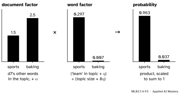
The Gibbs update for “team” in d7. The document leans slightly to baking, but the word overwhelmingly to sports, and the product decides.
Counts without this word. In d7, ball is in sports and bake and flour in baking: \({n_{d,\text{sports}} = 1}\), \({n_{d,\text{baking}} = 2}\). “Team” appears four more times in d1 to d3, all in sports: \({n_{\text{sports},\text{team}} = 4}\) and \({n_{\text{baking},\text{team}} = 0}\). The sports topic holds 12 words from d1 to d3 plus ball from d7, so 13; the baking topic 12 plus 2, so 14.
Normalise.\({0.4457 / (0.4457 + 0.0169) = 0.963}\). The sampler puts “team” in sports with probability 0.963 and in baking with 0.037. The baking topic is not impossible, because \(\eta\) gives an unseen word a small share.
Code
From scratch: a collapsed Gibbs sampler for the corpus. After a burn-in of 100 sweeps it averages the estimates over 1000 more, relabelling each sample so that topic 0 is the one holding more copies of “team” (the Pitfalls say why).
import numpy as npdocs = ["ball goal team goal", "team match ball team", "goal match team ball","flour sugar bake oven", "bake oven flour bake", "sugar flour bake oven","team bake ball flour"]words =sorted({w for d in docs for w in d.split()})K, V, alpha, eta =2, len(words), 0.5, 0.1def gibbs(sweeps=1100, burn=100, seed=0): rng = np.random.default_rng(seed) tokens = [[words.index(w) for w in d.split()] for d in docs] z = [rng.integers(K, size=len(t)) for t in tokens] # a random start ndk, nkw, nk = np.zeros((len(docs), K)), np.zeros((K, V)), np.zeros(K)for d, (td, zd) inenumerate(zip(tokens, z)):for w, k inzip(td, zd): ndk[d, k] +=1; nkw[k, w] +=1; nk[k] +=1 theta, beta = np.zeros((len(docs), K)), np.zeros((K, V))for sweep inrange(sweeps):for d, (td, zd) inenumerate(zip(tokens, z)):for i, w inenumerate(td): k = zd[i] ndk[d, k] -=1; nkw[k, w] -=1; nk[k] -=1# leave word i out p = (ndk[d] + alpha) * (nkw[:, w] + eta) / (nk + V * eta) k = rng.choice(K, p=p / p.sum()) zd[i] = k ndk[d, k] +=1; nkw[k, w] +=1; nk[k] +=1if sweep >= burn: order = np.argsort(-nkw[:, words.index("team")]) # align the labels theta += ((ndk + alpha) / (ndk.sum(axis=1, keepdims=True) + K * alpha))[:, order] beta += ((nkw + eta) / (nk[:, None] + V * eta))[order] kept = sweeps - burnreturn theta / kept, beta / kepttheta, beta = gibbs()for k, name inenumerate(["topic 0", "topic 1"]):print(name, [words[j] for j in np.argsort(-beta[k])[:4]])print("theta, sports share:", theta[:, 0].round(3))
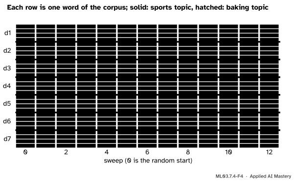
A document of four words in one topic would have \({\hat\theta = (4 + 0.5)/(4 + 1) = 0.9}\); the averages sit a little below that because the chain sometimes moves a word. The mixed d7 is close to one half. The topic of every word during the first sweeps of a run looks like this:
ML03.7.4-F4
A Gibbs chain on the corpus from a random start. The pure documents sort themselves out in a few sweeps; d7’s words stay split between the topics, and some keep moving, which is what an equal share looks like.
The library’s LatentDirichletAllocation fits the same model by variational inference, not by sampling. Its doc_topic_prior is \(\alpha\) and its topic_word_prior is \(\eta\); it takes documents as rows of counts.
from sklearn.decomposition import LatentDirichletAllocationfrom sklearn.feature_extraction.text import CountVectorizervectorizer = CountVectorizer()counts = vectorizer.fit_transform(docs)topic_model = LatentDirichletAllocation(n_components=2, doc_topic_prior=0.5, topic_word_prior=0.1, learning_method="batch", max_iter=200, random_state=0)shares = topic_model.fit_transform(counts)vocab = vectorizer.get_feature_names_out()for row in topic_model.components_:print("topic:", [str(vocab[j]) for j in np.argsort(-row)[:4]])print("d7 shares:", shares[6].round(3), " d1 shares:", shares[0].round(3))new = topic_model.transform(vectorizer.transform(["goal oven"]))print("a new document, 'goal oven':", new.round(3))
The new document gets shares at once, and they are even, since one word comes from each topic.
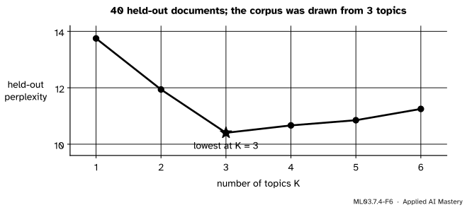
Choosing K. Hold some documents back and compute the perplexity, the exponential of minus the log-likelihood per held-out word: lower means the model predicts unseen text better. scikit-learn’s perplexity uses its variational lower bound in place of the exact log-likelihood, so its values are approximate. On a synthetic corpus drawn from the topic model itself with three topics, the held-out perplexity is lowest at \({K = 3}\).
rng = np.random.default_rng(0)true_beta = rng.dirichlet(np.full(30, 0.1), size=3) # 3 topics over 30 wordstrue_theta = rng.dirichlet(np.full(3, 0.3), size=200) # 200 documentscorpus = np.array([rng.multinomial(40, t @ true_beta) for t in true_theta])train, test = corpus[:160], corpus[160:]perplexity = {}for k inrange(1, 7): m = LatentDirichletAllocation(n_components=k, learning_method="batch", max_iter=30, random_state=0).fit(train) perplexity[k] =float(m.perplexity(test))print({k: round(v, 2) for k, v in perplexity.items()})
Held-out perplexity for \({K = 1}\) to 6. Too few topics cannot explain the words; too many spread the evidence thin.
Explore
The module’s interactive, the factor explorer, sits in lesson ML03.7.2. The NMF parts it finds at rank 2 are the same two groups of words that the topic model finds here.
Pitfalls
ML03.7.4-F5
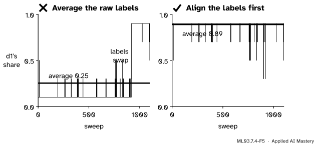
Wrong beside right. Partway through this run the sampler swapped the two topic labels. Averaging raw shares across the swap gives d1 a meaningless 0.25; aligning the labels first gives 0.89.
“Average every sample of the chain to get the topics.”
Topic numbers mean nothing: swapping the labels of two topics gives exactly the same probability, and a long chain can wander from one labelling to the other. Griffiths and Steyvers warn that estimates cannot be combined across samples for this reason. Align the labels of each sample (here by the topic holding “team”), or use a single sample, or average only quantities that do not depend on the labels.
“scikit-learn’s topic model is a Gibbs sampler.”
LatentDirichletAllocation uses variational Bayes, an optimisation that gives deterministic answers for a fixed random_state. Its numbers will be close to, not equal to, a sampler’s: the pure documents get \({(4 + 0.5)/(4 + 1) = 0.9}\) there, to three places, against about 0.89 above. Its components_ are pseudo-counts; divide each row by its sum to get \({\vect{\beta}_k}\).
“The K with the lowest perplexity gives the best topics.”
Perplexity measures how well the model predicts held-out words, not whether a person can name its topics. Use it to rule out bad choices of \(K\), then read the top words of each topic before you trust them.
Check yourself
Recall
1. List the three steps of the topic model’s generative story.
Show answer
Each topic draws \({\vect{\beta}_k \sim \text{Dirichlet}(\eta)}\); each document draws \({\vect{\theta}_d \sim \text{Dirichlet}(\alpha)}\); each word draws a topic \({z \sim \vect{\theta}_d}\) and then a word from \({\vect{\beta}_z}\).
2. What does a Dirichlet concentration below 1 do to the topic shares?
Show answer
It pushes them towards the corners and edges of the simplex: most documents use one or a few topics.
3. Write the collapsed Gibbs update for the topic of word \(i\).
4. What does the prior on the topic shares fix that pLSA got wrong?
Show answer
A new document draws its own shares from the prior, so the model gives it a probability, and the number of parameters no longer grows with the number of documents.
5. What is perplexity, and which way is better?
Show answer
The exponential of minus the log-likelihood per held-out word. Lower is better.
Exercises
1.★ In the worked example’s state, resample the topic of “bake” in d7. Find the probability of the baking topic.
Show solution
Without this word, d7 has team and ball in sports (2) and flour in baking (1). “Bake” appears elsewhere 4 times, all in baking (d4 once, d5 twice, d6 once). The baking topic then holds \({12 + 1 = 13}\) words and sports \({12 + 2 = 14}\). So
and the baking topic has probability 0.963: the mirror image of the worked example.
2.★★ For a symmetric Dirichlet on \({K = 2}\) topics, write the density of \({\theta = \theta_{d1}}\) (the other share is \({1 - \theta}\)) for \({\alpha = 1}\) and for \({\alpha = 2}\). Check that each integrates to 1.
Show solution
The density is \({\Gamma(2\alpha)/\Gamma(\alpha)^2\;\theta^{\alpha - 1}(1 - \theta)^{\alpha - 1}}\). For \({\alpha = 1}\) it is \({\Gamma(2)/\Gamma(1)^2 = 1}\), the uniform density, with integral 1. For \({\alpha = 2}\) it is \({\Gamma(4)/\Gamma(2)^2\,\theta(1 - \theta) = 6\theta(1 - \theta)}\), and \({\int_0^1 6(\theta - \theta^2)\,d\theta = 6(\tfrac12 - \tfrac13) = 1}\).
Show that this implies the document factor of the Gibbs update for \({K = 2}\). Hint: integrate the shares out of \({p(\vect{z}_d \mid \vect{\theta}_d)}\) with and without word \(i\).
Show solution
With counts \({n_1, n_2}\) of the two topics in document \(d\), integrating the shares out against the Dirichlet gives
Adding word \(i\) to topic 1 raises \(n_1\) and the total by one. Dividing by the value without it and using \({\Gamma(x + 1) = x\Gamma(x)}\) leaves \({(n_1 + \alpha)/(n_1 + n_2 + 2\alpha)}\). The denominator is the same for either topic, so the update is proportional to \({n_{dk}^{-i} + \alpha}\).
Summary card
Every document draws its own topic shares from a Dirichlet.
Gibbs:\(P(z_i = k)\) is proportional to \({(n_{dk}^{-i} + \alpha)}\) times \({(n_{kw}^{-i} + \eta)/(n_k^{-i} + V\eta)}\).
Choose K by held-out perplexity; align labels before averaging samples.
Sources and next steps
Sources. Each was opened and checked against this lesson on 15 November 2026.
D. M. Blei, A. Y. Ng and M. I. Jordan, Latent Dirichlet Allocation, JMLR 3 (2003), 993 to 1022. Section 3: the generative process and the Dirichlet density (equation 1); section 4.3: the comparison with pLSI; section 5.4: smoothing with an exchangeable Dirichlet prior \(\eta\) on the topics; section 7.1: perplexity as the exponential of minus the held-out log-likelihood per word.
T. L. Griffiths and M. Steyvers, Finding scientific topics, PNAS 101, suppl. 1 (2004), 5228 to 5235. Equations 2 and 3: the integrals over the topic and share distributions; equation 5: the full conditional for one word’s topic; equations 6 and 7: the estimates, with a footnote that such estimates cannot be combined across samples because the topics are not identifiable.
scikit-learn, Latent Dirichlet Allocation, User Guide section 2.5.8 (online and batch variational Bayes; \(\alpha\) is doc_topic_prior and \(\eta\) is topic_word_prior), and the API page of LatentDirichletAllocation (components_ as pseudo-counts, perplexity).
Next. Topic models are one of the tools for exploring text in A01, Natural language processing foundations, and the sampling behind the Gibbs update is treated in full in ML05.9, Sampling-based inference. The next module, ML03.8, turns to estimating a density directly.