HDBSCAN runs DBSCAN at every eps at once, as single linkage on the mutual reachability distance, then keeps the clusters that last longest. Build the spanning tree, condense it with min_cluster_size, score clusters by stability, and solve the blobs that defeated DBSCAN.
ML03.3.4L2 Intermediate30 minIn review (what this means)
The maths and code on this page are checked by automated tests on every change, but an independent reader has not signed it off yet. Spot a mistake or a confusing step? Tell us.
Compute the mutual reachability distance and explain how it pushes sparse points away from everyone.
Prove that cutting the minimum spanning tree of mutual reachability at eps gives the DBSCAN* clusters at eps.
Condense the hierarchy with min_cluster_size and select clusters by their stability, worked by hand on the twelve points.
Fit sklearn.cluster.HDBSCAN, read labels_ and probabilities_, and use it on clusters of different density.
The question
OPTICS showed every density at once, but you still had to read the valleys: by eye, or with a steepness threshold you had to choose. Can an algorithm pick the clusters itself, each at the density that suits it, given only the smallest group you would call a cluster?
From the last lesson
1. What is the reachability distance of \(\vect{o}\) from a core point \(\vect{p}\)?
Show answer
The larger of the core distance of \(\vect{p}\) and the distance \(d(\vect{p}, \vect{o})\): the smallest \(\varepsilon\) at which \(\vect{o}\) is directly density-reachable from \(\vect{p}\).
2. On a reachability plot, what does a horizontal line at \(\varepsilon\) give?
Show answer
The DBSCAN clustering for that \(\varepsilon\), up to a few border points: each run of bars below the line is a cluster.
Intuition
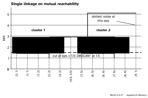
Run DBSCAN at a huge \(\varepsilon\) and everything is one cluster. Lower \(\varepsilon\) slowly: the cluster sheds its loneliest points, splits, shrinks, and in the end every point is alone. Record that history as a tree. A cluster that survives over a long range of \(\varepsilon\) is real; one that flickers in and out is an accident of one setting.
ML03.3.4-F1
The history of DBSCAN over every \(\varepsilon\), for the twelve points with min_samples = 4. Read any horizontal line as one run of DBSCAN* (DBSCAN without border points). The two shaded groups exist from \(\varepsilon = 2.915\) down to 1.414; HDBSCAN keeps them.
That is HDBSCAN, from Campello, Moulavi and Sander (2013). It needs two numbers you can choose without seeing a single distance: min_samples, as in DBSCAN, and min_cluster_size, the smallest group worth calling a cluster.
Build it up
Step 1. DBSCAN without border points. HDBSCAN uses DBSCAN*: clusters are the connected pieces of the core graph, and every non-core point is noise. Dropping border points removes the order dependence of lesson ML03.3.2 and makes the clusters nest neatly as \(\varepsilon\) changes.
Step 2. One distance for both conditions. Two points are in the same DBSCAN* cluster at \(\varepsilon\) when a chain joins them in which every point is core (\({\operatorname{core} \le \varepsilon}\)) and every step is short (\({d \le \varepsilon}\)). Fold the three conditions into one number, the mutual reachability distance:
In a dense region \(d_{\text{mr}}\) is about the plain distance. A sparse point has a large core distance, and all its distances are raised to at least that: it is pushed away from everyone.
ML03.3.4-F2
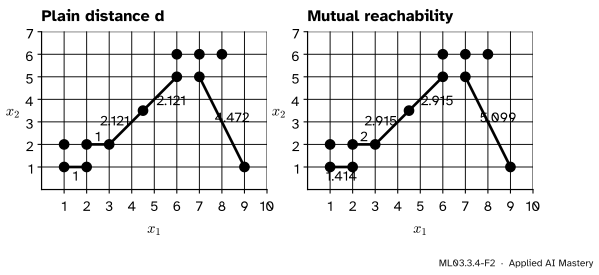
Within a square the distance rises only from 1 to 1.414; the bridge’s links rise from 2.121 to its core distance 2.915, and the link to \((9, 1)\) from 4.472 to 5.099.
Step 3. A spanning tree. Treat \(d_{\text{mr}}\) as edge weights on the complete graph and take its minimum spanning tree: the cheapest set of \(n - 1\) edges that connects every point.
Step 4. Cut it from the top. Remove the tree’s edges from the heaviest down: this is the single-linkage hierarchy of lesson ML03.2.4, run on \(d_{\text{mr}}\). Removing every edge heavier than \(\varepsilon\) leaves the DBSCAN* clusters at \(\varepsilon\).
Step 5. Condense. Most splits are a cluster shedding one or two points. With min_cluster_size\(= s\), a split counts only if both pieces have at least \(s\) points; otherwise the small piece’s points fall out as noise and the cluster carries on under the same name. The result, the condensed tree, has few clusters, each with a birth and with points leaving it over time.
Step 6. Keep the clusters that last. Measure density by \(\lambda = 1/\varepsilon\). A cluster’s stability adds up how long each of its points stayed in it; choose the non-overlapping set of clusters with the largest total stability.
The formal statement
Fix min_samples\(= m\) and write \(\operatorname{core}(\vect{x}) = d_{m-1}(\vect{x})\), so that \(\vect{x}\) is core at \(\varepsilon\) exactly when \(\operatorname{core}(\vect{x}) \le \varepsilon\) (lesson ML03.3.2).
NoteTheorem: single linkage on mutual reachability is DBSCAN* at every eps
For every \(\varepsilon\), delete from a minimum spanning tree of \(d_{\text{mr}}\) every edge heavier than \(\varepsilon\), and call a point with \(\operatorname{core} > \varepsilon\) noise. The pieces that remain, apart from the noise points, are the DBSCAN* clusters at \(\varepsilon\).
Proof. A maximum is at most \(\varepsilon\) exactly when each of its terms is, so
The right-hand side says: \(\vect{a}\) and \(\vect{b}\) are both core at \(\varepsilon\) and within \(\varepsilon\), that is, they are joined by an edge of the core graph. So the graph whose edges are the pairs with \(d_{\text{mr}} \le \varepsilon\) is the core graph, and its connected pieces are the DBSCAN* clusters. A point with \(\operatorname{core} > \varepsilon\) has \(d_{\text{mr}} > \varepsilon\) to everyone and is alone: noise.
Finally, two points are connected through pairs with \(d_{\text{mr}} \le \varepsilon\) exactly when they are connected in the spanning tree without its edges heavier than \(\varepsilon\), the property of minimum spanning trees behind lesson ML03.2.4 (proved below). \(\square\)
Go deeper: why the spanning tree keeps every connection below eps
Let \(T\) be a minimum spanning tree of a weighted graph, and suppose \(\vect{a}\) and \(\vect{b}\) are joined by some path of edges of weight at most \(\varepsilon\). The tree path between them could, in principle, use a heavier edge \(e\). Remove \(e\) from \(T\): the tree falls into two parts, with \(\vect{a}\) in one and \(\vect{b}\) in the other. The light path from \(\vect{a}\) to \(\vect{b}\) must cross between the parts somewhere, along an edge \(f\) of weight at most \(\varepsilon\), lighter than \(e\). Then \(T\) with \(e\) replaced by \(f\) is a spanning tree of smaller total weight, which contradicts minimality. So every edge of the tree path weighs at most \(\varepsilon\). The converse is clear, since the tree’s edges are edges of the graph.
Stability. Write \(\lambda = 1/\varepsilon\). A cluster \(C\) of the condensed tree is born at \(\lambda_{\text{birth}}(C)\), when it splits off its parent, and each of its points \(\vect{x}\) leaves it at some \(\lambda_{\vect{x}}\), by falling out or because \(C\) splits or ends. Following Campello et al., its stability is
A cluster scores highly when many points stay in it over a long range of densities.
Selection (excess of mass, scikit-learn’s default "eom"). Work up from the leaves, which start selected. At each cluster compare \(S(C)\) with the best total of its descendants: if \(S(C)\) is at least as large, select \(C\) and drop them; otherwise keep them and pass their total up. The root may not win unless allow_single_cluster=True.
Worked example
The twelve points with min_samples = 4 and min_cluster_size = 4.
Mutual reachability. The core distances are the 3-distances: 1.414 for six corners, 1 for \((2, 2)\) and \((7, 6)\), 2 for \((3, 2)\) and \((8, 6)\), 2.915 for the bridge, 5.099 for \((9, 1)\). So two adjacent corners of a square are \(\max(1.414, 1.414, 1) = 1.414\) apart; \((2, 2)\) and \((3, 2)\) are 2; the bridge and \((3, 2)\) are \(\max(2.915, 2, 2.121) = 2.915\), and so are the bridge and \((6, 5)\); \((7, 5)\) and \((9, 1)\) are \(\max(1.414, 5.099, 4.472) = 5.099\).
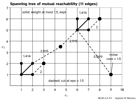
The spanning tree. Its eleven edges: three of weight 1.414 inside each square, one of weight 2 to each of \((3, 2)\) and \((8, 6)\), two of weight 2.915 through the bridge, and one of 5.099 to \((9, 1)\). Any direct link between the groups is dearer: \((3, 2)\) to \((6, 5)\) costs \(\max(2, 1.414, 4.243) = 4.243\). Ties make the tree not unique (the bridge is 2.915 from five points), but every choice has these weights and the same hierarchy; the figure shows SciPy’s.
ML03.3.4-F3
Deleting the dashed edges, those heavier than 1.5, leaves the two squares: DBSCAN* at \(\varepsilon = 1.5\), where \((3, 2)\) and \((8, 6)\) are noise rather than border points.
The condensed tree, from \(\lambda = 0\) down.
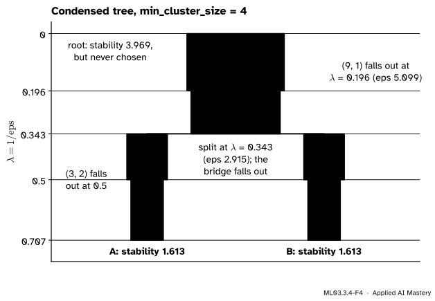
At \(\lambda = 1/5.099 = 0.196\) the edge to \((9, 1)\) goes. A piece of one point is smaller than 4, so \((9, 1)\) falls out and the root carries on with 11 points.
At \(\lambda = 1/2.915 = 0.343\) both bridge edges go. The pieces are the lower five, the upper five and the bridge alone. Two pieces have at least 4 points: a true split. Clusters A and B are born; the bridge falls out.
At \(\lambda = 1/2 = 0.5\) the edges to \((3, 2)\) and \((8, 6)\) go; each falls out of its cluster.
At \(\lambda = 1/1.414 = 0.707\) the square’s three edges go together and A ends with its last four points; B likewise.
ML03.3.4-F4
The condensed tree with min_cluster_size = 4. Column widths count the points still in each cluster. A and B each have stability 1.613.
Stabilities. For A, born at 0.343: \((3, 2)\) stays until 0.5 and the four corners until 0.707, so
\(B\) has the same shape, so \(S(B) = 1.613\). The root, born at 0, keeps \((9, 1)\) until 0.196 and the other eleven until 0.343: \({0.196 + 11 \times 0.343} = 3.969\).
Selection. A and B are leaves, so both are selected. Their parent is the root, which is not allowed to win by default; the answer is A and B. (With allow_single_cluster=True the root’s 3.969 beats the 3.227 of A and B together, and the answer is one cluster of eleven with \((9, 1)\) as noise.) Points that fell out of a selected cluster, like \((3, 2)\), keep its label: two clusters of five, as DBSCAN found. Each point also gets a membership strength, probabilities_: for these points it is the point’s \(\lambda_{\vect{x}}\) over the largest \(\lambda\) in its cluster, so \((3, 2)\) gets \({0.5 / 0.707} = 0.707\) and the corners 1.
The bridge. Its two edges tie at 2.915. Removed together, they leave the bridge alone: noise. scikit-learn 1.9 returns it instead as A’s weakest member, with probability \({0.343 / 0.707} = 0.49\), as if it left A at the moment A was born. The other ten points do not depend on the tie.
Code
From scratch as far as the spanning tree, then the cut at \(\varepsilon = 1.5\), checked against DBSCAN’s core points.
Three clusters: each tight blob whole, and 92 of the sparse blob’s points together (two join a tight blob, six are noise). Each blob was found at its own density.
Explore
The module’s DBSCAN explorer is in lesson ML03.3.2. Sweep its eps from large to small with min_samples = 4: one group above 2.915, two below, and below 1.414 the outer corners stop being core, where the condensed tree ends each cluster.
Pitfalls
ML03.3.4-F5
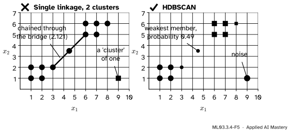
Wrong beside right. Single linkage on plain distances chains the groups through the bridge; HDBSCAN keeps them apart and calls \((9, 1)\) noise.
“HDBSCAN is just single linkage, so it chains like single linkage.”
Single linkage on plain distances merges the groups at 2.121 and calls \((9, 1)\) a cluster of one. Mutual reachability raises the links of sparse points, so a chain of strays joins groups only at a large \(\varepsilon\), and min_cluster_size turns one-point splits into points falling out.
“min_samples and min_cluster_size are the same knob.”
min_samples sets the core distances, and so how readily points become noise; min_cluster_size decides which splits count. scikit-learn sets min_samples to min_cluster_size by default: on the blobs, 20 instead of 5 raises the noise from 6 points to 16.
“probabilities_ are probabilities of belonging to the cluster.”
They are relative strengths: the density \(\lambda_{\vect{x}}\) up to which a point stayed, as a share of the largest \(\lambda\) reached in its cluster. They are not calibrated and do not sum to 1 over clusters.
Check yourself
Recall
1. Write the mutual reachability distance between \(\vect{a}\) and \(\vect{b}\).
Show answer
The largest of the two core distances and the distance between the points:
5. On the twelve points with min_samples = 4 and min_cluster_size = 4, what are the stabilities of the two clusters and why does the root, with a larger stability, not win?
Show answer
Each has stability 1.613; the root has 3.969. By default the root is never selected; allow_single_cluster=True lets it win.
Exercises
1.★ Two points are 1 apart, with core distances 0.5 and 2. A third point is 3 from the first and has core distance 0.5. Give the two mutual reachability distances from the first point.
Show solution
To the second point: \(\max(0.5, 2, 1) = 2\). The second point is sparse, so its link is raised to its core distance.
To the third point: \(\max(0.5, 0.5, 3) = 3\). Both are dense, and the plain distance decides.
2.★★ In a condensed tree, cluster P (stability 2.0) splits into Q (0.8) and R (0.9), and Q later splits into Q1 (0.6) and Q2 (0.7). Q1, Q2 and R have no children, and P is not the root. Which clusters does the excess-of-mass rule select?
Show solution
Work from the leaves up. Q1, Q2 and R are leaves and start selected.
At Q: its own stability is 0.8, its children’s total is \({0.6 + 0.7} = 1.3\). The children win: keep Q1 and Q2 and pass up 1.3 as Q’s value.
At P: its own stability is 2.0; the best its descendants achieve is \({1.3 + 0.9} = 2.2\). The descendants win again.
The selection is Q1, Q2 and R. (With R at 0.6 the descendants would total 1.9, and P would win.)
3.★★★ Show that the mutual reachability distance obeys the triangle inequality:
The left side is the largest of three terms. It is enough to show each is at most the right side, which we call \(R\). Every term of a maximum is at most the maximum, so \(\operatorname{core}(\vect{a}) \le d_{\text{mr}}(\vect{a}, \vect{b})\) and \(\operatorname{core}(\vect{c}) \le d_{\text{mr}}(\vect{b}, \vect{c})\), and also \(d(\vect{a}, \vect{b}) \le d_{\text{mr}}(\vect{a}, \vect{b})\) and \(d(\vect{b}, \vect{c}) \le d_{\text{mr}}(\vect{b}, \vect{c})\). Distances are not negative, so:
by the triangle inequality for \(d\), the distance \(d(\vect{a}, \vect{c})\) is at most \({d(\vect{a}, \vect{b}) + d(\vect{b}, \vect{c})}\), which is at most \(R\).
All three terms are at most \(R\), so their maximum is too.
Summary card
Run DBSCAN* at every eps as single linkage on mutual reachability, and keep the clusters that last.
ML03.3.4-F1
The hierarchy of every eps.
Mutual reachability.\(d_{\text{mr}}(\vect{a}, \vect{b})\) is the largest of the two core distances and \(d(\vect{a}, \vect{b})\).
Theorem. Cut the spanning tree of \(d_{\text{mr}}\) at \(\varepsilon\): the pieces are DBSCAN* at \(\varepsilon\).
Condense with min_cluster_size; score each cluster by its stability\(S(C)\); keep the most stable set.
In code.HDBSCAN(min_cluster_size, min_samples): labels_ with \(-1\) for noise, probabilities_.
Sources and next steps
Sources. Each was opened and checked against this lesson on 15 November 2026.
Ricardo J. G. B. Campello, Davoud Moulavi and Jörg Sander, Density-based clustering based on hierarchical density estimates, PAKDD 2013, Lecture Notes in Computer Science 7819, pages 160 to 172; repository record with abstract. The abstract states the method: a cluster hierarchy, a simplified tree of significant clusters, a stability measure, and an optimal selection of the most stable flat partition. The full text is not open; the details were checked in the next two sources.
scikit-learn developers, User Guide, section 2.3.8 HDBSCAN, version 1.9: the core distance to the min_samples-th neighbour counting the point itself, the mutual reachability distance, connected components of the trimmed graph as DBSCAN*, and the minimum spanning tree cut from its heaviest edges; and the sklearn.cluster.HDBSCAN API page: min_samples defaults to min_cluster_size, allow_single_cluster=False, the "eom" selection, labels_ and probabilities_.
How HDBSCAN works, documentation of the hdbscan library (scikit-learn-contrib): mutual reachability, the spanning tree, condensing with a minimum cluster size (points “falling out”), \(\lambda = 1/\text{distance}\), the stability \(\sum (\lambda_p - \lambda_{\text{birth}})\) and the bottom-up selection rule.
Next. Gaussian mixtures (module ML03.4) model each cluster as a density with a formula, and anomaly detection (module ML03.9) turns “noise” into a score.