When reference labels exist, compare a clustering with them through the contingency table, without caring how clusters are numbered. Purity, the Rand index over pairs, the adjusted Rand index that scores chance as 0, and mutual information with its normalised and adjusted forms.
ML03.10.2L2 Intermediate25 minIn review (what this means)
The maths and code on this page are checked by automated tests on every change, but an independent reader has not signed it off yet. Spot a mistake or a confusing step? Tell us.
Build the contingency table of two labellings and compute purity from it, and say why purity rewards splitting.
Count the pairs on which two labellings agree and compute the Rand index from the table.
Derive the expected pair count under random labelling and use it to compute the adjusted Rand index.
Compute the mutual information of two labellings and explain what normalising and adjusting it fix.
Compare clusterings of load_iris with scikit-learn’s external indices and interpret the scores.
The question
Iris comes with species labels. k-means finds three clusters and numbers them 0, 1 and 2 in whatever order it likes. How do you score the clusters against the species, when cluster 0 need not mean species 0, the counts need not match, and even a random labelling agrees with the truth on many points?
From the last lesson
1. What is the silhouette of the bridge point \({(4, 4)}\) in the best two-cluster split of the nine points?
Show answer
\({a} = {2.958}\), \({b} = {3.571}\), so \({s} = {(3.571 - 2.958)/3.571} = {0.172}\), the lowest of the nine.
2. Why did all three internal indices prefer k-means on the moons?
Show answer
They reward compact, round clusters. Each moon is long and curved, so DBSCAN’s correct clusters have large distances within them and score worse.
Intuition
Comparing a clustering with known groups is comparing two labellings of the same points. The names of the labels carry no meaning: renaming the clusters must not change the score. What does carry meaning is which points share a label. So count overlaps, not names.
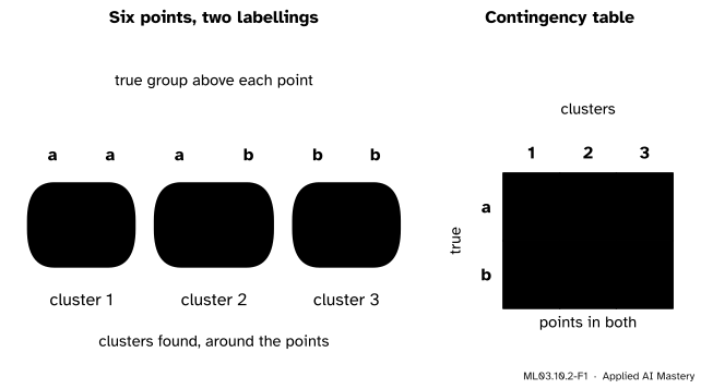
ML03.10.2-F1
Six points with two labellings: true groups \(a\) and \(b\), and three clusters found. The contingency table counts the points in each (group, cluster) pair. Renaming the clusters only reorders its columns.
Every external index in this lesson is computed from this table alone. A perfect clustering puts exactly one non-zero entry in every row and every column. Here group \(a\) is split over clusters 1 and 2, and cluster 2 mixes the two groups.
Build it up
Step 1. The table. Call the true labelling \(U\), with groups \({U_1, \dots, U_R}\), and the clustering \(V\), with clusters \({V_1, \dots, V_C}\). Entry \(n_{ij}\) counts the points in both \(U_i\) and \(V_j\). The row sums \(a_i\) are the group sizes and the column sums \(b_j\) the cluster sizes.
Step 2. Purity. Give each cluster the label of its largest group, and count the points that then match: purity\(= {\tfrac{1}{n}\sum_j \max_i n_{ij}}\). Here \({(2 + 1 + 2)/6 = 0.833}\). It is easy to read, but splitting can only help it: a cluster of one point is always pure.
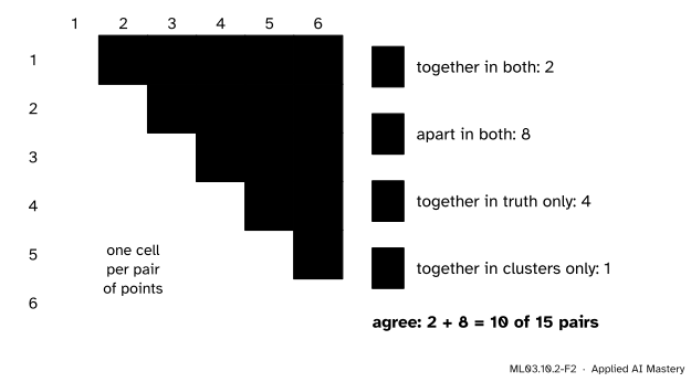
Step 3. Pairs. Take any two points. Each labelling either puts them together or apart, so the pair falls into one of four kinds.
ML03.10.2-F2
The 15 pairs of the six points, one cell each. The labellings agree on a pair when both put it together (2 pairs) or both put it apart (8 pairs), and disagree on the other 5.
Step 4. The Rand index. The share of pairs on which the two labellings agree is the Rand index: here \({(2 + 8)/15 = 0.667}\). Unlike purity it punishes splitting, since a split separates pairs that the truth keeps together.
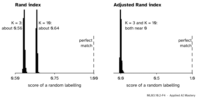
Step 5. The catch. Is \(0.667\) good? Label the 150 iris flowers at random with three clusters and the Rand index is still about \(0.56\), because most pairs are “apart” in both labellings by luck. A useful score needs a baseline: what does chance give?
The formal statement
Pair counts from the table. Two points in cell \({(i, j)}\) are together in both labellings, so the number of such pairs, the index, is \({\sum_{ij} \binom{n_{ij}}{2}}\). Likewise \({\sum_i \binom{a_i}{2}}\) pairs are together in \(U\) and \({\sum_j \binom{b_j}{2}}\) together in \(V\).
NoteThe adjusted Rand index (Hubert and Arabie, 1985)
Under random labelling with the same group and cluster sizes,
Write \(I\) for the index, \(E\) for this expectation and \({M} = {\tfrac12\big[\sum_i \binom{a_i}{2} + \sum_j \binom{b_j}{2}\big]}\). Then
\[
\mathrm{ARI} = \frac{I - E}{M - E} .
\]
Why the expectation is that product. Keep \(U\) fixed and shuffle the points among the clusters of \(V\), keeping the cluster sizes: this is the permutation model. The index counts, over the \({P_U} = {\sum_i \binom{a_i}{2}}\) pairs that are together in \(U\), those that are also together in \(V\). After the shuffle, any fixed pair of points lands on a uniformly random pair of positions, so it is together in \(V\) with probability
the share of all pairs that lie inside a cluster of \(V\). The expected count is a sum of \(P_U\) indicators, each with mean \(q\). By linearity of expectation it is \({P_U\,q}\), which is the formula.
Why \(M\). The index cannot exceed \({\sum_i \binom{a_i}{2}}\) or \({\sum_j \binom{b_j}{2}}\), so it is at most the smaller of the two, and their mean \(M\) is a convenient upper bound that is reached when the two labellings are identical. So ARI is \(1\) for identical labellings, \(0\) on average for random ones, and can be negative when agreement is worse than chance.
ML03.10.2-F4
Random labellings of iris. The Rand index of pure chance sits near \(0.56\) with 3 clusters and climbs to \(0.64\) with 10; the adjusted index sits at \(0\) for both.
Mutual information. Read the table as a joint distribution, \({p_{ij} = n_{ij}/n}\), with margins \(a_i/n\) and \(b_j/n\). The entropy\({H(U)} = {-\sum_i (a_i/n) \ln (a_i/n)}\) measures how uncertain a random point’s group is (M09.1 treats it fully). The mutual information measures how much knowing the cluster reduces that uncertainty (M09.2):
\({\E[\mathrm{MI}]}\) is again taken under the permutation model; Vinh, Epps and Bailey give it as a closed sum, and for a small table it can be found by averaging over every shuffle. scikit-learn uses the arithmetic mean of the two entropies by default.
Worked example
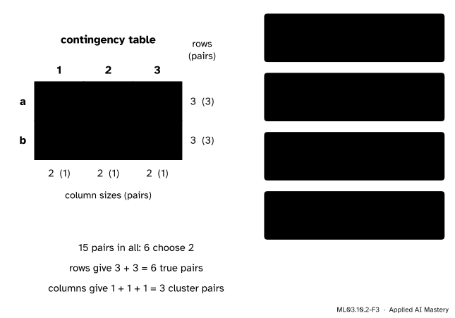
The six points: truth \({(a, a, a, b, b, b)}\), clusters \({(1, 1, 2, 2, 3, 3)}\).
Pairs. The cells \({2, 1, 0}\) and \({0, 1, 2}\) give \({I} = {\binom22} + {\binom22} = {2}\). The rows, of size 3 each, give \({P_U = 3 + 3 = 6}\); the columns, of size 2 each, give \({P_V = 1 + 1 + 1 = 3}\); and there are \({\binom62 = 15}\) pairs.
Rand index. Agreeing pairs are the \(2\) together in both and those apart in both, \({15 - 6 - 3 + 2 = 8}\), so \({\mathrm{RI}} = {10/15} = {0.667}\).
Adjusted.\({E = 6 \times 3/15 = 1.2}\) and \({M = (6 + 3)/2 = 4.5}\), so
The adjusted Rand index of the six points, from the table. The raw agreement of 2 pairs is compared with the 1.2 that chance would give and with the most possible, 4.5.
Mutual information. Only the two cells with \({n_{ij}} = {2}\) and the two with \({n_{ij}} = {1}\) count. For a cell with 2 points, \({n\,n_{ij}/(a_i b_j)} = {6 \cdot 2/(3 \cdot 2)} = {2}\); for a cell with 1 point it is \({6 \cdot 1/(3 \cdot 2) = 1}\), whose logarithm is 0. So
The groups are equal halves, \({H(U) = \ln 2 = 0.693}\); the clusters are equal thirds, \({H(V) = \ln 3 = 1.099}\). Then \({\mathrm{NMI}} = {0.462/0.896} = {0.516}\). Averaging MI over all \(720\) shuffles gives \({\E[\mathrm{MI}] = 0.277}\), and
From scratch: the table, the pair counts, the ARI, and MI with its expectation found by brute force.
import itertoolsfrom math import comb, logimport numpy as npfrom sklearn.metrics import (adjusted_mutual_info_score, adjusted_rand_score, mutual_info_score, normalized_mutual_info_score, rand_score)from sklearn.metrics.cluster import contingency_matrixdef table(u, v): T = np.zeros((u.max() +1, v.max() +1), int)for i, j inzip(u, v): T[i, j] +=1return Tdef ari(u, v): T = table(u, v); n = T.sum() I =sum(comb(int(x), 2) for x in T.ravel()) PU =sum(comb(int(x), 2) for x in T.sum(1)); PV =sum(comb(int(x), 2) for x in T.sum(0)) E = PU * PV / comb(int(n), 2); M = (PU + PV) /2return (I - E) / (M - E), I, E, Mdef mi(u, v): T = table(u, v); n = T.sum(); a = T.sum(1); b = T.sum(0)returnsum(T[i, j] / n * log(n * T[i, j] / (a[i] * b[j]))for i inrange(len(a)) for j inrange(len(b)) if T[i, j])def entropy(u): p = np.bincount(u) /len(u)return-sum(x * log(x) for x in p if x >0)u = np.array([0, 0, 0, 1, 1, 1]); v = np.array([0, 0, 1, 1, 2, 2])score, I, E, M = ari(u, v)mean_H = (entropy(u) + entropy(v)) /2E_mi = np.mean([mi(u, v[list(p)]) for p in itertools.permutations(range(6))])print(table(u, v));print(f"I = {I}, E = {E:.1f}, M = {M}, ARI = {score:.3f}")print(f"MI = {mi(u, v):.3f}, NMI = {mi(u, v) / mean_H:.3f}, E[MI] = {E_mi:.3f}, "f"AMI = {(mi(u, v) - E_mi) / (mean_H - E_mi):.3f}")
[[2 1 0]
 [0 1 2]]
I = 2, E = 1.2, M = 4.5, ARI = 0.242
MI = 0.462, NMI = 0.516, E[MI] = 0.277, AMI = 0.299
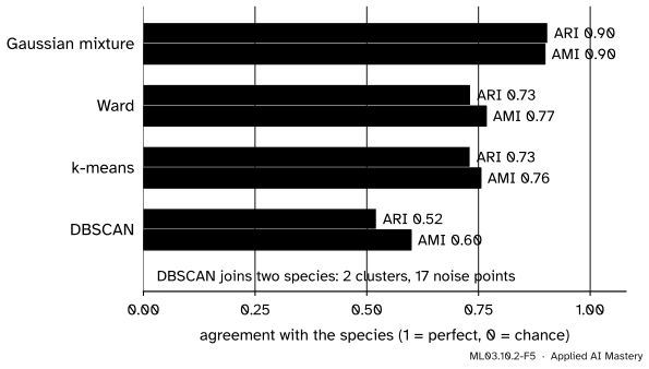
Now four clusterings of iris, each asked for three groups (DBSCAN with its defaults), against the species. The Gaussian mixture’s numbers depend on its random starts, so they are checked to two decimals.
from sklearn.cluster import DBSCAN, AgglomerativeClustering, KMeansfrom sklearn.datasets import load_irisfrom sklearn.mixture import GaussianMixtureX, y = load_iris(return_X_y=True)found = {"k-means": KMeans(3, n_init=10, random_state=0).fit_predict(X),"Ward": AgglomerativeClustering(3, linkage="ward").fit_predict(X),"Gaussian mixture": GaussianMixture(3, n_init=5, random_state=0).fit_predict(X),"DBSCAN": DBSCAN(eps=0.5, min_samples=5).fit_predict(X)}for name, z in found.items():print(f"{name:17s} RI {rand_score(y, z):.3f} ARI {adjusted_rand_score(y, z):.3f} "f"NMI {normalized_mutual_info_score(y, z):.3f} AMI {adjusted_mutual_info_score(y, z):.3f}")print(contingency_matrix(y, found["k-means"]))
k-means           RI 0.880  ARI 0.730  NMI 0.758  AMI 0.755
Ward              RI 0.880  ARI 0.731  NMI 0.770  AMI 0.767
Gaussian mixture  RI 0.957  ARI 0.904  NMI 0.900  AMI 0.898
DBSCAN            RI 0.772  ARI 0.521  NMI 0.604  AMI 0.599
[[ 0 50  0]
 [48  0  2]
 [14  0 36]]
ML03.10.2-F5
Four clusterings of iris against the species. The mixture, whose ellipses fit the elongated species, agrees best; DBSCAN’s defaults merge versicolor and virginica.
Finally, chance. Draw random labellings and the Rand index stays far above zero, while the adjusted indices do not.
rng = np.random.default_rng(0)for K in (3, 10): draws = [rng.integers(0, K, len(y)) for _ inrange(200)]print(f"K = {K}: mean RI {np.mean([rand_score(y, z) for z in draws]):.3f}, "f"mean ARI {np.mean([adjusted_rand_score(y, z) for z in draws]):+.3f}, "f"mean AMI {np.mean([adjusted_mutual_info_score(y, z) for z in draws]):+.3f}")
K = 3: mean RI 0.557, mean ARI -0.001, mean AMI -0.001
K = 10: mean RI 0.637, mean ARI -0.000, mean AMI -0.001
Explore
The cluster scorecard in lesson ML03.10.3 prints the adjusted Rand index against the groups each point set was drawn from. On three blobs, compare the ARI at \({K} = {2}\), \(3\) and \(4\); on touching blobs, watch the ARI fall below 1 even at the true \(K\).
Pitfalls
ML03.10.2-F6
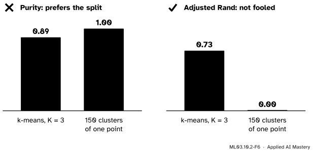
Wrong beside right. Purity gives 150 clusters of one point a perfect \(1.00\), higher than any real clustering. The adjusted Rand index gives them \(0\): they agree with the species on no pair.
“Match each cluster to its majority species and report the accuracy.”
That is purity, and it is biased towards many small clusters: in the limit of one point per cluster it is perfect. It also ignores how a group is split. Use the adjusted Rand index or AMI, which punish splitting and score chance as \(0\).
“A Rand index of 0.6 is a decent agreement.”
Random labels of iris already score \(0.56\) with three clusters and \(0.64\) with ten. The unadjusted Rand index and NMI have no fixed baseline, and their chance level rises with the number of clusters (Vinh, Epps and Bailey show the same for NMI). Quote the adjusted versions.
“The species are the true clusters, so the highest ARI wins.”
Reference labels are one grouping of interest, not the only structure in the data. Versicolor and virginica overlap in these four measurements, so DBSCAN’s two groups are a defensible reading of the data even though they score \(0.52\) against the species. And labels used to choose a clustering method can no longer judge it fairly: keep some aside, as with a test set (ML01.2).
Check yourself
Recall
1. Why can a clustering not be scored by plain accuracy against the labels?
Show answer
Cluster numbers are arbitrary, so cluster 0 need not correspond to label 0, and the numbers of clusters and labels may differ. The score must not change when clusters are renamed.
2. What does the contingency table hold?
Show answer
In row \(i\) and column \(j\), the number \(n_{ij}\) of points that are in group \(U_i\) and cluster \(V_j\). Its row sums are the group sizes and its column sums the cluster sizes.
3. What does the Rand index count?
Show answer
The share of all pairs of points on which the two labellings agree: together in both, or apart in both.
4. What is the expected number of pairs together in both labellings under random labelling?
Show answer
\({\sum_i \binom{a_i}{2} \sum_j \binom{b_j}{2} / \binom{n}{2}}\): the pairs together in \(U\) times the chance that a random pair is together in \(V\).
5. What values can the adjusted Rand index take, and what do \(0\) and \(1\) mean?
Show answer
At most \(1\), for identical labellings; \(0\) on average for random labellings; negative values when agreement is worse than chance.
Exercises
1.★ Truth \({(a, a, b, b)}\) and clusters \({(1, 1, 1, 2)}\). Find the contingency table, the Rand index and the purity.
Show solution
Table: row \(a\) is \({(2, 0)}\) and row \(b\) is \({(1, 1)}\). There are \({\binom42} = {6}\) pairs. Together in both: \({\binom22} = {1}\) (the two \(a\) points). Together in the truth: \({1} + {1} = {2}\). Together in the clusters: \({\binom32} = {3}\). Apart in both: \({6 - 2 - 3} + {1} = {2}\). So RI \(= {(1 + 2)/6} = {0.5}\). Purity: cluster 1 has majority \(a\) with 2 points, cluster 2 has one \(b\), so \({(2 + 1)/4 = 0.75}\).
2.★★ For the same labellings, compute the adjusted Rand index.
Show solution
\({I} = {1}\), \({P_U} = {2}\), \({P_V} = {3}\), \({\binom42} = {6}\). So \({E = 2 \times 3/6 = 1}\) and \({M = (2 + 3)/2 = 2.5}\). Then \({\mathrm{ARI}} = {(1 - 1)/(2.5 - 1)} = {0}\): the clustering agrees with the truth on exactly as many pairs as chance would.
3.★★★ Show that the mutual information of two labellings is \(0\) when every cell satisfies \({n_{ij} = a_i b_j / n}\), and explain what that condition says about the clusters.
Show solution
In every term, \({n\,n_{ij}/(a_i b_j)} = {n \cdot (a_i b_j/n)/(a_i b_j)} = {1}\), and \({\ln 1 = 0}\), so every term of MI vanishes. The condition says that \({n_{ij}/b_j = a_i/n}\): inside every cluster, the share of group \(i\) is the same as in the whole data set. The clusters then carry no information about the groups, which is what MI \(= {0}\) should mean. (A cell with \({n_{ij} = 0}\) contributes 0 by convention, and the condition only allows it when \({a_i b_j} = {0}\).)
Summary card
Compare labellings through their contingency table, and always against chance.
ML03.10.2-F1
Count overlaps, not names.
Purity.\({\tfrac1n \sum_j \max_i n_{ij}}\); rises to 1 with one point per cluster.
Rand index. Share of pairs on which the labellings agree.
AMI.\({(\mathrm{MI} - \E[\mathrm{MI}])/(\bar H - \E[\mathrm{MI}])}\), the same idea for information.
Six points. RI \(0.667\), ARI \(0.242\), NMI \(0.516\), AMI \(0.299\).
Sources and next steps
Sources. Each was opened and checked against this lesson on 15 November 2026.
Nguyen Xuan Vinh, Julien Epps and James Bailey, Information Theoretic Measures for Clusterings Comparison: Variants, Properties, Normalization and Correction for Chance, Journal of Machine Learning Research 11 (2010), 2837 to 2854. Section 2 sets out the contingency table (Table 1) with row sums \(a_i\) and column sums \(b_j\), the four kinds of pairs, the Rand index and the adjusted Rand index of Hubert and Arabie (1985), and the entropies and mutual information. Section 4.1 describes the permutation model with fixed cluster sizes, gives the expected mutual information (equation 2), the general adjusted form “(Index − Expected Index)/(Max Index − Expected Index)” (equation 3), and the AMI. The opening of Section 4 shows that the chance level of RI and NMI rises with the number of clusters.
scikit-learn developers, User Guide, Section 2.3.11 Clustering performance evaluation, version 1.9. Section 2.3.11.1 defines RI and ARI and warns that the unadjusted Rand index is “often close to 1.0” for very different clusterings; 2.3.11.2 defines MI, NMI and AMI; 2.3.11.8 shows the contingency matrix with this lesson’s six-point example; 2.3.11.9 the pair confusion matrix. That average_method defaults to the arithmetic mean is read from the library itself.