An anomaly detector gives every point a score of strangeness and flags the highest. Meet the kinds of anomaly, outlier against novelty detection, z-scores, the Mahalanobis distance with its chi-square cut-off, masking and the robust fix.
ML03.9.1L2 Intermediate30 minIn review (what this means)
The maths and code on this page are checked by automated tests on every change, but an independent reader has not signed it off yet. Spot a mistake or a confusing step? Tell us.
Tell point, contextual and collective anomalies apart, and outlier detection from novelty detection.
Explain why every detector is a score followed by a threshold, and how an expected contamination sets the threshold.
Compute the Mahalanobis distance by hand and derive the chi-square cut-off for a Gaussian in the plane.
Explain masking, and fix it with a minimum covariance determinant estimate (EllipticEnvelope).
Use a density estimate from ML03.4 or ML03.8 as a score, and say what it assumes.
The question
A bank sees ten million card payments a day. A few hundred are fraud, and nobody has marked which. A factory logs a thousand sensor readings a minute, and the one that warns of a failing bearing carries no label either. You cannot train a classifier without examples of the thing you look for. How can you rank every point by how strange it is, so that people look at the top of the list first?
Intuition
An anomaly is a point that does not fit the pattern the rest of the data follow. Without labels, “does not fit” has to be measured from the data alone, and every method in this module does it in the same two steps.
ML03.9.1-F1
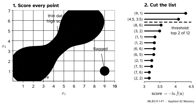
A detector in two steps. First give every point a score of strangeness; here it is minus the log of a density estimate, high where the data are thin. Then cut the ranked list: flag the top 2 of 12.
First, a score: a number for each point, larger for stranger points. Second, a threshold: flag every point whose score is at least \(c\). The picture shows both on the twelve points of the course. The two points that sit in thin data, the bridge \((4.5, 3.5)\) and the far point \((9, 1)\), get the highest scores.
The threshold usually comes from a guess about how much of the data is strange, the contamination. If you expect one point in six, flag the top sixth of the list. The detectors of this module differ only in the score: distance from a fitted Gaussian here, a ratio of local densities in ML03.9.2, the length of a random path in ML03.9.3, and a reconstruction error or a learned boundary in ML03.9.4.
Build it up
Step 1. Three kinds of anomaly. Chandola, Banerjee and Kumar (2009, section 2.2) sort them by what makes them strange.
ML03.9.1-F2
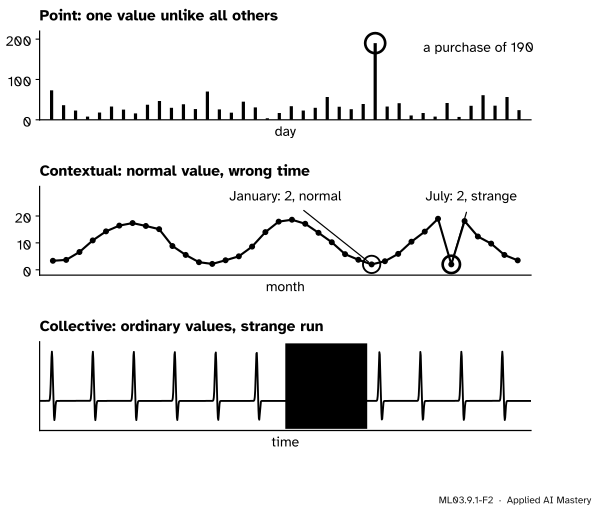
A point anomaly is strange on its own. A contextual anomaly is an ordinary value at the wrong time or place. A collective anomaly is a run of ordinary values that is strange as a whole.
A purchase of 190 among purchases below 70 is a point anomaly. A temperature of 2 degrees is normal in January and strange in July: a contextual anomaly, where time is the context. A heartbeat that stays flat for two beats is a collective anomaly; no single value in it is unusual. This module treats point anomalies. Context and runs come back with time series in S07.10.
Step 2. Outliers or novelties. In outlier detection the anomalies sit inside the data you fit, and the method must find them in spite of their pull. In novelty detection the training data are clean, and you ask whether a new point is strange. scikit-learn’s user guide (section 2.7) keeps the two apart, and some of its estimators change behaviour between them.
Step 3. Why labels are rare. Fraud, machine faults and network intrusions are rare, labelling them takes an expert, and new kinds keep appearing that no past label covers (Chandola et al., section 2.3). So the detectors here use no labels to fit. When a few labels exist, they are kept to judge a detector, as ML03.9.4 does.
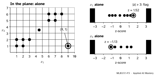
Step 4. One feature at a time. The simplest score is the z-score of S01.4.4, \({z = (x - \bar{x})/s}\), with a flag at \({\abs{z} > 3}\). Run it on each feature of the twelve points and the far point \((9, 1)\) is never flagged.
ML03.9.1-F3
Each feature alone, \((9, 1)\) is ordinary: \(z = 1.52\) for \(x_1\) and \(z = -1.13\) for \(x_2\). It is strange only as a pair of values, because large \(x_1\) goes with large \(x_2\) everywhere else.
Its \(x_1 = 9\) is the largest value but not far out, and its \(x_2 = 1\) is shared by two other points. What is strange is the combination: everywhere else, large \(x_1\) comes with large \(x_2\). A score for points in the plane must know how the features vary together.
Step 5. Distance in units of the data’s own spread. Fit one Gaussian to the data: a mean \(\vect{\mu}\) and a covariance \(\mat{\Sigma}\). Measure each point’s distance from the mean along the directions the data stretch in, counting a step along a long axis of the cloud as less than a step across it. That is the Mahalanobis distance, and its level sets are the ellipses of ML03.4.4.
ML03.9.1-F4
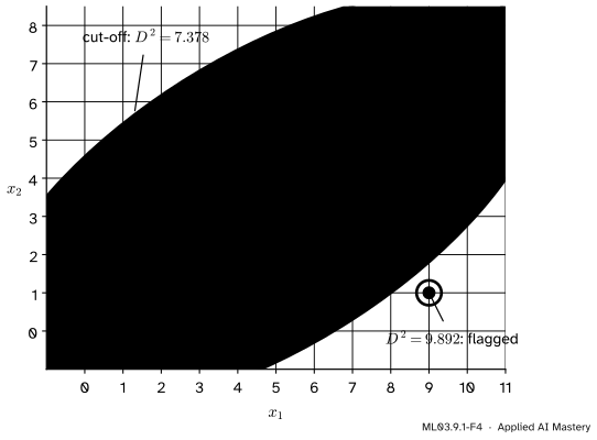
One Gaussian fitted to the twelve points. The far point lies outside the cut-off ellipse, at \({D^2 = 9.892}\). The bridge point sits on the mean, at \({D^2 = 0.025}\): to this model it is the most typical point of all.
The far point is caught. The bridge is not: it sits between two groups, exactly where one Gaussian puts its peak. A score is only as good as the model of “normal” behind it.
The formal statement
NoteDefinition: the Mahalanobis distance
For a distribution with mean \(\vect{\mu}\) and covariance \(\mat{\Sigma}\) in \(\R^d\), the squared Mahalanobis distance of a point \(\vect{x}\) is
The last two terms are the same for every point. So ranking points by \(D^2\) is ranking them by low Gaussian density. Any density estimate can play the same part: the score \({-\ln \hat f(\vect{x})}\) with \(\hat f\) a kernel estimate (ML03.8) or a Gaussian mixture (ML03.4), as in the anchor figure.
The cut-off, derived for the plane. Suppose the data really are Gaussian. Write \({\mat{\Sigma} = \mat{Q}\mat{\Lambda}\mat{Q}\T}\) by the spectral theorem (M03), and whiten: \({\vect{z} = \mat{\Lambda}^{-1/2}\mat{Q}\T(\vect{x} - \vect{\mu})}\). Then \(\vect{z}\) has mean \(\vect{0}\) and covariance \(\mat{I}\), its two coordinates are independent standard normals, and
the squared radius of \(\vect{z}\). The density of \(\vect{z}\) is \({\tfrac{1}{2\pi} e^{-r^2/2}}\). In polar coordinates the area element is \(r\,dr\,d\varphi\), so the chance of landing beyond radius \(\sqrt{c}\) is
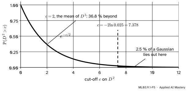
To flag a share \(\alpha\) of Gaussian points, set \({e^{-c/2} = \alpha}\), so \({c = -2\ln\alpha}\). For \(\alpha = 0.025\) this gives \({c = 7.378}\). In \(d\) dimensions \(D^2\) is a sum of \(d\) squared standard normals, the chi-square distribution with \(d\) degrees of freedom, and scipy.stats.chi2.ppf(0.975, d) gives the cut-off.
ML03.9.1-F5
For a Gaussian in the plane the share of points with \({D^2 > c}\) is \(e^{-c/2}\). The cut-off 7.378 leaves 2.5 % outside.
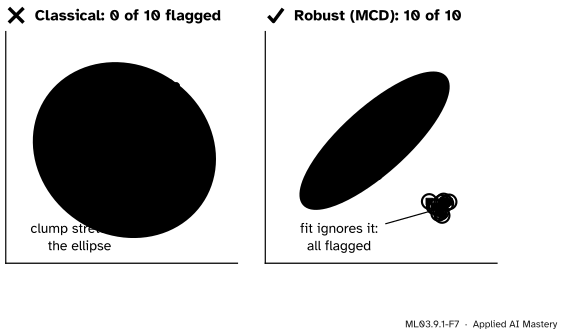
Masking, and the robust fix. The mean and covariance are estimated from the same data that hold the outliers. A clump of outliers drags the mean towards itself and stretches the covariance until its own points look ordinary. This is masking: the outliers hide themselves.
NoteDefinition: the minimum covariance determinant estimate
Among all subsets of \(h\) points, take the one whose sample covariance has the smallest determinant. Its mean and (rescaled) covariance are the MCD estimates of location and scatter.
Why the determinant? The ellipse \({D^2 \le 1}\) has half-axes \(\sqrt{\lambda_1}\) and \(\sqrt{\lambda_2}\), the square roots of the eigenvalues of \(\mat{\Sigma}\), so its area is \({\pi\sqrt{\lambda_1\lambda_2} = \pi\sqrt{\det\mat{\Sigma}}}\). The smallest determinant picks the \(h\) points that fit inside the tightest ellipse. Points far from the bulk of the data would stretch that ellipse, so they tend to be left out, as long as there are fewer of them than the \({n - h}\) points the estimate may drop. scikit-learn’s MinCovDet finds it with the FastMCD algorithm of Rousseeuw and Van Driessen, taking \(h\) at least about half the data, and EllipticEnvelope thresholds the robust \(D^2\) at the contamination you give.
Worked example
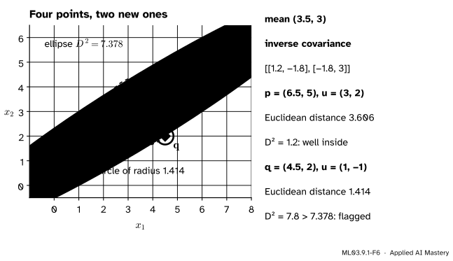
Take the four points of M03, \((0, 1)\), \((3, 2)\), \((4, 4)\) and \((7, 5)\), and two new ones, \(\vect{p} = (6.5, 5)\) and \(\vect{q} = (4.5, 2)\). Which is stranger?
Mean and covariance. The mean is \((3.5, 3)\). Divide the centred scatter matrix of M03 by \({n - 1 = 3}\):
Euclidean distance calls \(\vect{q}\) closer; the Mahalanobis distance calls it far stranger, because it steps across the line the data follow.
Result:\(\vect{p}\) is 3.606 from the mean in Euclidean distance but has \({D^2 = 1.2}\), deep inside the cloud’s ellipse. \(\vect{q}\) is only 1.414 away, yet \({D^2 = 7.8 > 7.378}\): it is flagged. (With four points the covariance is a rough estimate; the arithmetic, not the verdict, is the point here.)
Code
From scratch on the twelve points: z-scores, the Mahalanobis distance with the maximum-likelihood covariance (divide by \(n\), as EmpiricalCovariance does), and the cut-off.
import mathimport numpy as npfrom scipy import statsX = np.array([(1, 1), (2, 1), (1, 2), (2, 2), (3, 2), (6, 5), (7, 5), (6, 6), (7, 6), (8, 6), (4.5, 3.5), (9, 1)], dtype=float)z = (X - X.mean(axis=0)) / X.std(axis=0, ddof=1) # s divides by n - 1, as in S01mu = X.mean(axis=0)Sigma = (X - mu).T @ (X - mu) /len(X)U = X - mud2 = np.einsum("ij,jk,ik->i", U, np.linalg.inv(Sigma), U)cut =-2* math.log(0.025)print("largest |z|:", np.abs(z).max().round(3), " z of (9, 1):", z[11].round(3))print("mean:", mu.round(3), " D^2 of bridge and (9, 1):", d2[10].round(3), d2[11].round(3))print("cut-off:", round(cut, 3), " scipy:", round(stats.chi2.ppf(0.975, 2), 3))print("flagged:", X[d2 > cut].tolist())
largest |z|: 1.515  z of (9, 1): [ 1.515 -1.13 ]
mean: [4.708 3.375]  D^2 of bridge and (9, 1): 0.025 9.892
cut-off: 7.378  scipy: 7.378
flagged: [[9.0, 1.0]]
No z-score can reach 3 by much here: among \(n\) values the largest possible \(\abs{z}\) is \({(n - 1)/\sqrt{n}}\) (S01.4.4), which is 3.175 for \(n = 12\). Now masking. Sixty correlated Gaussian points and a clump of ten outliers, seeded; the classical fit against the robust one.
clump flagged, classical: 0 of 10; largest clump D^2: 6.6
clump flagged, robust:    10 of 10; normal points flagged: 0
EllipticEnvelope with contamination 10/70 flags the clump: True
EllipticEnvelope fits MinCovDet, and its score_samples is minus the robust squared distance. Last, a density as the score: a kernel estimate with bandwidth 1 (ML03.8).
from sklearn.neighbors import KernelDensityscore =-KernelDensity(bandwidth=1.0).fit(X).score_samples(X)top2 = np.argsort(-score)[:2]print("highest scores:", X[top2].tolist(), score[top2].round(3))
This module’s interactive, the isolation forest explorer, lives in ML03.9.3. Its contamination slider is the threshold of this lesson: slide it and watch the flagged set grow from the top of the ranked list.
Pitfalls
ML03.9.1-F7
Wrong beside right. The classical fit lets the clump stretch the ellipse until none of its ten points crosses the cut-off. The minimum covariance determinant fit ignores the clump and flags all ten.
“Fit the mean and covariance to all the data, then flag what lies far out.”
The outliers are in the data you fit, so they move the very estimate that should expose them. One far point inflates the spread; a clump can hide completely. Use a robust estimate (MinCovDet, EllipticEnvelope) or train on data known to be clean (novelty detection).
“A Mahalanobis distance works on any data.”
It assumes one elliptical cloud. On the twelve points it calls the bridge the most typical point, because one Gaussian puts its peak between the two groups. scikit-learn’s documentation warns that the MCD is not meant for multi-modal data. For several groups, use a mixture (ML03.4) or a local method (ML03.9.2).
“The detector tells me how many anomalies there are.”
The contamination is your assumption. Set it to 1/6 and one point in six is flagged, whatever the data. Report the ranked scores, and treat the threshold as a budget for how many cases people can check.
“An outlier is an error, so delete it.”
Sometimes it is a typo; sometimes it is the fraud you were paid to find. Check flagged points, and never delete one silently (S01.4.4).
Check yourself
Recall
1. Name the two steps every detector in this module takes.
Show answer
It computes a score of strangeness for every point, then flags the points whose score is at least a threshold \(c\), often set so that a chosen share (the contamination) is flagged.
2. What is the difference between outlier detection and novelty detection?
Show answer
In outlier detection the anomalies are inside the training data. In novelty detection the training data are clean, and the question is whether a new point is strange.
3. Why is \((9, 1)\) not flagged by z-scores on the twelve points?
Show answer
Each of its coordinates is ordinary on its own (\(z = 1.52\) and \(-1.13\)). It is strange only as a combination, because elsewhere large \(x_1\) goes with large \(x_2\).
4. For a Gaussian in the plane, what share of points has \({D^2 > c}\), and what cut-off leaves 2.5 % outside?
Show answer
The share is \(e^{-c/2}\), so the cut-off is \({c = -2\ln 0.025 = 7.378}\).
5. What is masking, and what fixes it?
Show answer
Outliers pull the mean and stretch the covariance that is fitted with them, so their own distance looks ordinary. A robust estimate such as the minimum covariance determinant, fitted on the tightest half of the data, fixes it.
Exercises
1.★ With the mean and inverse covariance of the worked example, compute \(D^2\) for \((2, 4)\) and for \((6, 2)\). Which of them does the cut-off 7.378 flag?
Show solution
With the inverse covariance, an offset \({\vect{u} = (u_1, u_2)}\) has
Both exceed 7.378, so both are flagged. Each lies off the line the four points follow.
2.★★ For a Gaussian in the plane, what cut-off on \(D^2\) flags 1 % of points? What share of points lies beyond \({D^2 = 4}\), the ellipse at “two standard deviations”?
Beyond \({D^2 = 4}\) lies \({e^{-4/2} = e^{-2} = 0.135}\), so 13.5 %. In one dimension, two standard deviations leave about 4.6 % outside; in the plane the same radius leaves almost three times as much, because the two directions each contribute.
3.★★★ Show that the Mahalanobis distance does not change when the data are rescaled or rotated: if every point is mapped to \({\mat{A}\vect{x} + \vect{b}}\) with \(\mat{A}\) invertible, then \(D^2\) of every point is the same as before.
Show solution
The new mean is \({\mat{A}\vect{\mu} + \vect{b}}\), so the new offset is \({\mat{A}\vect{x} + \vect{b} - \mat{A}\vect{\mu} - \vect{b} = \mat{A}(\vect{x} - \vect{\mu})}\). The new covariance is \({\mat{A}\mat{\Sigma}\mat{A}\T}\), with inverse \({(\mat{A}\T)^{-1}\mat{\Sigma}^{-1}\mat{A}^{-1}}\). Write \({\vect{u} = \vect{x} - \vect{\mu}}\). Then the new squared distance is
Robust. Minimum covariance determinant against masking: EllipticEnvelope(contamination=...).
Density. Score \({-\ln \hat f(\vect{x})}\) with a kernel estimate or a mixture.
Sources and next steps
Sources. Each was opened and checked against this lesson on 15 November 2026.
Varun Chandola, Arindam Banerjee and Vipin Kumar, Anomaly detection: a survey, ACM Computing Surveys 41(3), article 15, 2009 (the authors’ page with the PDF). Section 2.2 defines point, contextual (with the temperature example) and collective anomalies (with the heartbeat example); section 2.3 explains why labels are scarce and costly.
scikit-learn developers, User Guide, section 2.7, Novelty and outlier detection, version 1.9: outlier against novelty detection, and the elliptic envelope as a robust covariance fit thresholded by Mahalanobis distance.
scikit-learn developers, User Guide, section 2.6.4, Robust covariance estimation: the empirical covariance is very sensitive to outliers; the minimum covariance determinant keeps a proportion \(h\) of good observations, and FastMCD (Rousseeuw and Van Driessen) computes it.